Tables in PDFs for RAG: Don’t Flatten the Grid

The number you need sits in a table, at the intersection of a row and a column. Flatten the PDF to text and that intersection is gone: the label lands in one place, the value in another, and the model is left guessing which number belongs to which row. Tables are where naive parsing quietly loses the answer.

This article is a bonus in Enterprise Document Intelligence, a series that builds an enterprise RAG system from four bricks. Tables in PDFs: a diagnostic and five composable operations that keep the grid, instead of a decision tree.

🧭 New to the series? Every article in this series sits on our two Towards Data Science author pages, Angela Shi and Kezhan Shi. That is the shortest way to see what is covered and where this one sits.

📓 Runnable companion notebooks are on GitHub: doc-intel/notebooks-vol1.

The standard RAG pipeline reads a PDF, chunks it into text, embeds the chunks, and retrieves the closest match. The pipeline handles bullet points and paragraphs fine. The moment the answer to a question lives inside a table cell, the standard pipeline starts hallucinating numbers, and often nobody notices until an auditor opens the source document.

This article is about why tables break enterprise RAG, and what to do instead. It is positioned as a bonus because tables touch all four bricks (document parsing, question parsing, retrieval, generation) and none of the main articles owns the topic alone. Article 5 mentions fitz.find_tables() without a strategy. Article 10 escalates adaptive parsing without a table-specific cascade. Article 15 (preparing the corpus) extracts fields from tables without saying how to retrieve from one. This bonus consolidates the fragments into one coherent treatment.

1. Why tables break the pipeline

A table in a PDF is not a table in the data sense. It is a set of rectangles drawn on a page, with text positioned in cells, often without explicit row or column markers. The parser has to reconstruct the grid from spatial geometry. Sometimes it succeeds and you get a clean DataFrame. Often it does not.

When it does not, three things go wrong at once. First, the row and column structure is lost, so the LLM downstream sees a stream of values with no relational meaning. Second, the header is often only on the first page of a multi-page table, so pages two onward become numerical noise. Third, the line-level citation discipline of Article 8 breaks down because there is no way to point at “row 47” when row 47 was never reconstructed as a row.

All three failures share a root. A table is data that someone put into a layout format because the distribution format required it. The expert who created the schedule knew it was data. The parser that flattens the table into text destroys what the producer of the document already had. The right move is not to handle tables better as text. It is to restore them to their native structured form as early as possible and treat them as data from then on.

2. Four ways to represent a table

The same table can live in the pipeline at four different levels of structure. Picking the right level for each table is the first design decision, before any operation runs. The four levels are not alternatives to argue between in the abstract. Each is the right answer for a specific combination of table size, schema stability, and question shape.

A. Row-as-line in line_df is the default. It is what the parser produces naturally, and it is enough for any question whose answer reads from the table the same way it reads from prose. Each row of the table becomes one row of line_df with _type="table" and the text rendered as a Markdown pipe row (| col1 | col2 | col3 |). The line keeps its bounding box on the page, so highlighting and citation work the same as for prose. Downstream bricks see “lines that happen to be Markdown-shaped” and never branch on table-ness. This is what the Azure Document Intelligence parser emits today. A question like “what is the deductible for property coverage?” is answered from the Markdown row directly, retrieved like any other line, cited like any other line. Most tables in mixed-content documents stop here, because no operation downstream needs to address the columns by name.

B. Separate table_df. When you need to operate on the 2D shape, you lift the table out of line_df into its own DataFrame, with column headers preserved as DataFrame columns and rows as DataFrame rows. The line_df keeps a placeholder line pointing at the table by id. Three operations require this: concatenating a table that continues across five pages with the header only on the first, projecting to two columns out of fourteen because the question asks about one year, filtering to the rows whose region matches the scope. None of these are possible at A. Once the table is flattened into Markdown rows, the columns are textually visible but no longer addressable.

C. Columnar extraction with named, typed columns. Some tables recur across documents in a stable shape: an insurance contract’s premium table, a financial statement’s income summary, a regulatory schedule with fixed fields. These are not “tables in a PDF” anymore. They are data that the producer happened to provide as PDF because PDF was the distribution format, and the document we read is a layout of data that already had columns and types before it became a PDF. The right move is to restore that original form. Lift the tables into a columnar store at ingestion time, indexed by document id and table id. The choice of storage engine is orthogonal: Parquet on disk, DuckDB for in-process queries, Postgres if the corpus warrants a real database. What matters is that columns are named (policy_number, start_date, premium_amount) and typed (date, decimal, varchar). Once that holds, the table is data. You query it with SQL, you join across documents, you aggregate. C is what unlocks corpus-level questions: “what are the total premiums across all my insurance contracts?” requires that every contract’s premium column maps to the same name and type, which is the guarantee C makes.

D. Columnar but heterogeneous. Sometimes you want corpus-level addressing but the tables resist a common schema: different vendors, different versions, different layouts of “the same” information. The content lands in a single text column next to its metadata (doc_id, page, table_id). You keep document-level retrieval and full-text search across the corpus, but the 2D structure is gone. D is the honest fallback when C’s preconditions are not met. It is rarely chosen proactively. It shows up when the team tried for C and could not normalize the schemas in the time available.

The dispatcher picks one level per table. Most stay at A. A few escalate to B when a continuation or a projection is needed. The ones that recur across documents in a known shape get promoted to C at ingestion time. The orphan recurring tables fall to D.

The dimensions that drive the choice are not mutually exclusive, which is why a linear decision tree fails. A native, well-parsed table can also be very long. A multi-page continuation can also live in a document where 80% of the volume is tabular. A table the parser failed on can also need column projection. Each real table sits at the intersection of three or four conditions, and the right answer is a small diagnostic per table plus a handful of idempotent operations that move tables between levels. That is what the next two sections describe.

3. The diagnostic: table_df_meta

For every table detected in a document, the diagnostic records five orthogonal properties. The result is a small DataFrame (one row per table) that the dispatcher reads to pick the representation level (A, B, C, or D) and, when the level is B, which operations to apply.

Parse quality: Three levels. Perfect: the parser returned a clean grid with consistent row and column counts (fitz.find_tables() on a native PDF with explicit table borders is the typical case). Partial: the parser returned cells but the grid is irregular (rows of different widths, missing cells, merged cells misinterpreted), and the words have known bounding boxes on the page. Failed: the parser found rectangles but no usable grid, the page is scanned, or OCR returned text without structural cues.

Size: The pair (n_rows, n_cols). The relevant threshold is “fits in the LLM context with the surrounding question and prompt overhead”. Above the budget, projection (O3) becomes mandatory; below, it is optional. The exact cell count depends on the model’s context window and how much of it the prose and the system prompt already eat; no fixed threshold travels well across deployments.

Header status: Three values. Present: the first row is detected as header (either by font weight, by border, or because its cells contain mostly short text while later rows contain numbers). Absent: no row qualifies, often because the producer relied on the first-page header to cover the next pages too. Continuation: the table is a continuation of a previous one and its real header lives on an earlier page.

Multi-page continuity: Three values. Autonomous: the table starts and ends on the same page. Continued-from-N: same column count, same column x-positions, no header on this page, suggesting this is a continuation of the table on page N. Continues-to-M: the table on this page ends at the bottom and the next page starts with a table of the same column structure with no header. The detection rule is geometric (column positions match within 5 pixels) plus a header check.

Document-level context: The ratio of total table area to total text area in the document. The three example documents in section 5 sit at 6%, 13%, and 26% respectively. A document that crosses roughly half its body area in tables is one where the right architecture stops being RAG-on-text-with-tables-as-a-special-case and becomes SQL-on-extracted-tables-with-text-as-annotation. The exact crossover is qualitative, not numeric; the diagnostic reports the ratio and the dispatcher reads it alongside the per-table fields.

These five columns of table_df_meta are independent. A native, partial-quality, large, headerless, multi-page table in a table-dominant document is a valid row. The dispatcher reads all five fields and composes the response.

4. Five composable operations

Each operation takes a table_df (or a collection of them) as input and returns a transformed table_df. Most stay within level B and produce a cleaner B; O4 is the one promotion from B to C (or D). They are idempotent: applying an operation that does not match its precondition is a no-op, so the composition is safe.

O1. Structural reconstruction from positions. Applies when parse quality is partial and word bounding boxes are available. The parser delivered cells but the grid is broken. The operation rebuilds the grid by clustering word positions into column bands (x-coordinate histogram peaks) and into row bands (y-coordinate gaps wider than line height). The cells then snap to the (column, row) grid. This can recover a clean table_df that the native parser missed (the Commodity column in section 5’s CMO example and the over-split overview in the NIST example are both O1 candidates). Cost: one geometric pass per page, negligible. Failure mode: irregular tables with merged cells across rows defeat the simple grid model and trigger O5.

O2. Multi-page concatenation with header propagation. Applies when multi-page continuity is continued-from-N or continues-to-M. The operation walks the consecutive tables, detects the run, copies the header from the first table of the run to the rows of the continuation tables, and emits a single concatenated table_df with a new column source_page to preserve provenance. The geometric continuity check (same column count, same x-positions within tolerance, headerless continuation) is the precondition. Without this operation, a 200-row schedule split across 8 pages produces 8 separate table_df objects of which 7 are semantically orphan.

O3. Question-driven projection. Applies when size exceeds the context threshold. Reads the question’s scope_filters and concept_keywords (Article 6) and projects the table to the columns whose headers match the question concepts, then filters the rows whose values match the scope filters. A 200-row, 20-column schedule asked “what is the premium for property coverage in California” gets projected to columns [coverage_type, state, premium] and filtered to rows where state = 'CA', returning maybe 4 rows to send to the LLM. This is the “filter before retrieval” of Article 17 (querying the corpus), applied at the table level inside one document.

O4. Columnar extraction (B → C, or B → D). Applies when the table recurs across documents in a known shape, or when the document is dominated by tables that share a schema. The operation lifts the table(s) into the columnar store described in section 2 (level C), indexed by document id and table id. Subsequent questions are dispatched to a SQL agent (the pattern of Article 17, querying the corpus) instead of the retrieve-and-generate pipeline: the LLM writes SQL, the engine executes, the LLM interprets the result. The promotion succeeds at level C when a common schema can be identified across the matching tables; it lands at D when the schemas resist normalization.

O5. Vision-LLM fallback. Applies when O1 has failed (or when parse quality is failed from the start). The operation renders the page region around the table as an image and sends it to a vision-capable LLM with a structured prompt asking for a JSON representation of the table. Cost: at least an order of magnitude more expensive than O1, which is a free local geometric pass. The exact cost depends on the model and the image size, but the gap is always wide enough that O5 must stay a fallback, not a default, or the cost compounds quickly across long documents.

The operations compose. A table that is partial + continued-from-3 + large + question requires filtering runs O1 then O2 then O3. A document that is table-dominant with continued tables runs O2 across all continuations, then O4 on the consolidated tables. The dispatcher picks the composition.

5. The dispatcher

The dispatcher reads table_df_meta and emits a sequence of operations per table (or per document, for O4). It is deterministic and small enough to fit in one Python file, consistent with the decide.py pattern of Article 13.

Before the three examples, one preliminary point that sits underneath all of them: the parser choice matters at least as much as the operation choice. The same page parsed by two different tools can land in very different diagnostic buckets, so the dispatcher’s first job is to decide which parser to invoke. Only then does the per-table operation composition come in.

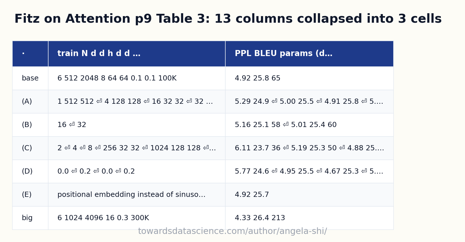
Take Table 3 of Attention Is All You Need (Vaswani et al. 2017; arXiv non-exclusive distribution license, declared on the arXiv abstract page; data/paper/1706.03762v7.pdf, page 9). The table is a hyperparameter-ablation grid with around twenty rows (header, base config, the (A)-(E) variation blocks, the big config) and thirteen columns (the variation label, the architecture hyperparameters N / d_model / d_ff / h / d_k / d_v, the regularization hyperparameters P_drop / ε_ls, train steps, and the metrics PPL / BLEU / params). It is exactly the kind of result table the article should reward the reader with. The article also parses World Bank CMO tables (CC BY 3.0 IGO) and uses Azure Document Intelligence (proprietary, Microsoft’s Online Services Terms) as one of the parsers.

Azure Document Intelligence on the same page recovers all 13 columns cleanly, including the sparse cells:

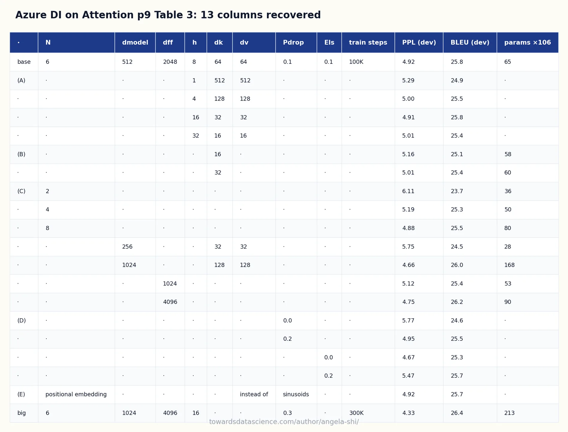
The diagnostic reads radically different on the same page. With Fitz: failed parse quality (Table 3 unrecoverable without O1+O5). With Azure DI: perfect. The Fitz pipeline has to do real work to salvage anything; the Azure pipeline gets clean table_df for free and skips O1-O5 entirely. Picking the right parser up front absorbs work the operations otherwise have to redo, and Azure’s per-page cost is small compared to a wrong answer on a hyperparameter-ablation question.

This is the spirit of Article 10’s adaptive escalation, restricted to the table case. Start with the cheap parser. When the diagnostic flags a hard table, escalate that table (or that page) to a stronger parser. The article 10 cascade and the B04 operation composition meet here: the parser cascade decides what level of table_df you start from; the operations decide what to do with it after.

Three examples on real public-domain documents. The scan results below come from a Fitz find_tables() sweep over every page; the parsed-table snapshots are produced by short chunks in this article’s source; both are reproducible.

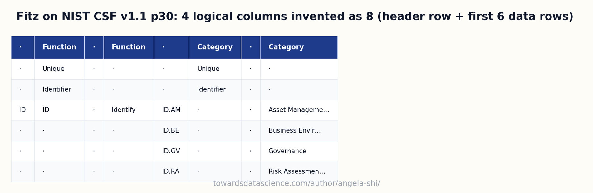
Example 1: NIST Cybersecurity Framework v1.1 (data/nist/NIST.CSWP.04162018.pdf, 55 pages, 28 tables found by Fitz, table-area ratio 26%). The Framework Core lives in Appendix A. Pages 30 to 32 hold three summary tables of decreasing width: the 26 by 8 overview shown above where Fitz inflates 4 logical columns into 8, then a 17 by 6 refinement on page 31, then an 8 by 4 split on page 32. From page 33 onward the main Core table runs across roughly 20 pages with a stable 4-column shape (Function, Category, Subcategory, Informative References) and 6 to 9 rows per page. Each continuation page carries a header row that Fitz detects, but the actual Function and Category values are blank on most rows because the producer only writes them once at the top of each block.

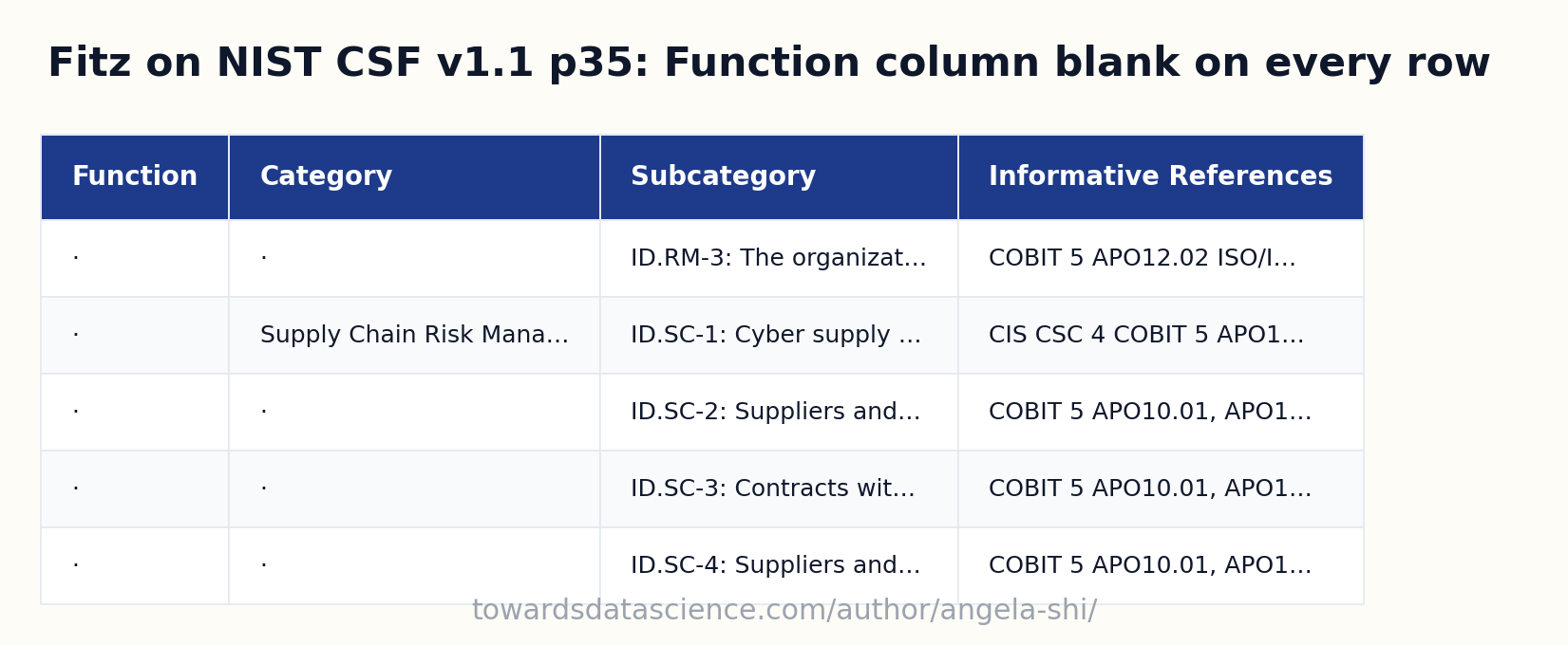
The diagnostic reads: partial parse quality on pages 30-32 (over-split grid), perfect on pages 33 onward, continued across the run, medium total size, document not table-dominant. Composition: [O1 on pages 30-32 to fold extra columns back to 4, O2 across pages 33-51 to forward-fill the missing Function and Category values and concatenate]. The result is one table_df with the full Framework Core (just over 100 subcategories) joined on (page_num, table_id). Without O1 + O2, a question like “what is subcategory PR.AC-3 about?” hits a continuation row where Function and Category are blank, and the LLM has no way to know the subcategory belongs to Protect → Identity Management and Access Control.

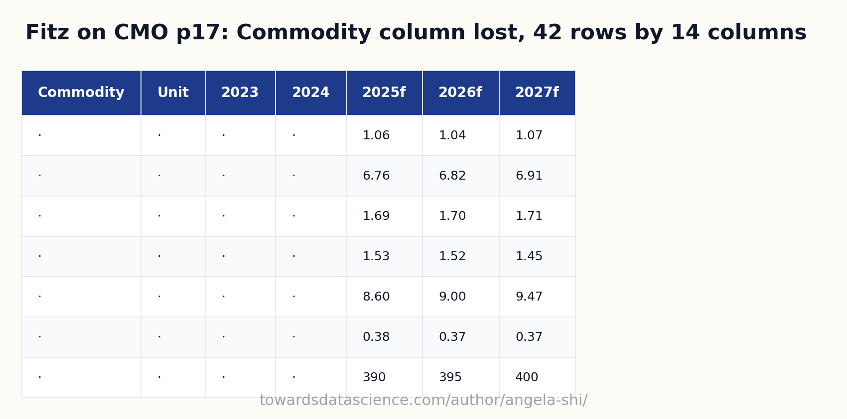
Example 2: World Bank Commodity Markets Outlook, October 2025 (data/cmo/CMO-October-2025.pdf, 66 pages, 38 tables found by Fitz, table-area ratio 6%, two-column document layout). The Price Forecasts table sits on page 17: 42 rows by 14 columns, one row per commodity, columns for historical years 2023-2024 and forecast years 2025-2027 across multiple revisions. Fitz captures the grid for the numeric block cleanly and completely drops the Commodity column; every row’s first cell comes back empty. The diagnostic reads: partial parse quality (label column missing), autonomous (single page), large size, document not table-dominant. Composition for a question like “what is the wheat price forecast for 2027?”: [O1 to recover the Commodity labels by clustering the left-margin word positions into a column band, then O3 to project to the (commodity=wheat, year=2027) cell]. Without O1, the LLM sees 42 rows of decimal numbers under “2027f” with no idea which one is wheat; O3 alone on the broken parse projects to the right year but cannot pick the right row.

The compositions are readable. An audit asking “why did this question return this row” walks the diagnostic, the operations applied in order, and the final table_df the LLM saw. Every step is logged. There is no hidden behavior.

6. The question type modulates the response

Once the right table_df is in hand (after diagnostic and composition), the question shape decides how the answer is produced. Three patterns.

Cell lookup: “What is the premium for property coverage in California?” The answer is one cell. The retrieval has filtered to one row; generation reads the cell and returns it with line-level citation back to the source page and row. The annotated PDF (Article 1’s highlighting) is reused: the cited cell gets the rectangle.

Range or column: “What are the deductibles for all coverage types?” The answer is a column slice. The retrieval has projected to the relevant columns and may return the whole table or a filter; generation returns the structured slice as a small markdown table embedded in the answer schema. Citation is at the table level rather than the cell.

Aggregate: “What is the total premium across all states?” The answer is a computation. The retrieval should not have happened in this branch at all. The dispatcher routes the question to the SQL agent (Article 17, querying the corpus), which writes SELECT SUM(premium) FROM schedule WHERE ..., executes, and the LLM interprets the scalar result. Citation is the SQL query plus the result, not a passage in the source document.

The question type is the modulator that determines the answer’s shape. It does not change the diagnostic or the operations; it only changes what gets returned once table_df is ready.

7. What stays out of this article

Several adjacent topics are real, important, and intentionally deferred to follow-up work to keep this bonus focused.

Cross-document table joining: “Compare the premium tables across all my insurance contracts.” This requires schema alignment across documents (the contract-A column premium_amount and contract-B column prime_annuelle need to map). It is corpus-level work, related to the field extraction of Article 15 (preparing the corpus) but applied to entire tables rather than scalar fields. Future series territory.

Purely visual tables: Bar charts presented as tables, color-coded matrices, infographic tables where the cell value is encoded by hue or size. These need vision-LLM treatment that goes beyond O5’s “reconstruct the grid” pattern. They need semantic interpretation of visual encodings. Follow-up work.

Complex OCR on tables: Scanned tables with hand-written annotations, tables in non-Latin scripts, tables in documents where the OCR layer is itself badly aligned with the visual layer. These need OCR-specific upstream work that is its own topic.

Long structured forms: Insurance application forms, tax returns, regulatory disclosure forms: these are form-shaped, not table-shaped. The distinction matters. A form has named fields with values; a table has rows of homogeneous structure. Forms get field extraction (Article 15, preparing the corpus). Tables get the treatment in this article. A document mixing both needs both treatments routed by the diagnostic.

8. Conclusion

The diagnostic-plus-composition pattern is the right response whenever a parsing problem is multi-dimensional and the dimensions are not mutually exclusive: a linear decision tree drops dimensions that did not make the cut, a diagnostic plus composable operations gives every artefact the treatment its specific properties call for. The expert who built the table knew it was data; the system’s job is to restore the table to its native structured form so the expert’s query lands on it. Handling tables as text, however carefully, drops the row-and-column structure that the expert’s question depends on.

9. Sources and further reading

The vision-based table-structure model behind most modern table extractors is Smock et al. (PubTables-1M / Table Transformer, CVPR 2022). The end-to-end PDF pipeline with explicit TableFormer module is Auer et al. (Docling Technical Report, 2024). The layout-detection benchmark behind table detectors is Pfitzmann et al. (DocLayNet, KDD 2022). The article’s framing: the diagnostic-plus-operations pattern, table_df_meta measures table properties (shape, header structure, merged cells, density), and five composable operations dispatch on those properties to do real work on the grid.

Earlier in the series:

• Document Intelligence: series intro. What the series builds, brick by brick, and in what order.

What works, what breaks

• Baseline Enterprise RAG, from PDF to highlighted answer. The four-brick pipeline end to end: PDF in, highlighted answer out.

• Embeddings Aren’t Magic: The Predictable Failure Modes of RAG Retrieval. Where embedding similarity wins (synonyms, typos, paraphrase), where it predictably breaks (unknown terms, negation, term-vs-answer relevance), and how to use it anyway.

• RAG is not machine learning, and the ML toolkit solves the wrong problem. Why chunk-size sweeps and finetuning optimize the wrong thing; route by question type instead.

• From regex to vision models: which RAG technique fits which problem. Two axes, document complexity and question control, that pick the technique for each case.

  • 10 common RAG mistakes we keep seeing in production. Ten production mistakes, organized brick by brick, with the fix for each.

Document parsing

• Building Document Structure with Loop Engineering: Recovering a PDF’s Outline from Body Typography for RAG. Rebuilding the outline from body typography when the PDF ships no contents page at all: six signals, one bounded loop.

• Before Full Agentic RAG: Know How You Decide, and the Parsing Methods You Pick From. The parsing methods as a catalogue, and the decision of which to run, before handing the loop to an agent.

Generation

• Most RAG Hallucinations Are Extraction Errors: Seven Patterns for a Typed Generation Contract. Seven recurring ways a model gets the extraction wrong, and the typed contract that catches each one.

• Loop engineering for RAG generation: an LLM cascade from a cheap local model up to a hosted flagship. Starting on a cheap local model and escalating only when the answer does not hold up, measured.

One-document pipelines

• Prompt Engineering Isn’t Enough: How Four Bricks of Context Engineering Stop RAG Hallucinations. Why a better prompt does not fix a wrong page, and what each of the four bricks contributes to the context instead.

• Cut an Enterprise RAG Pipeline’s Latency and Cost by Calling the LLM Less, Not by Buying a Faster Model. Cutting a pipeline’s latency and cost by calling the model less often and cheaper, not by buying a faster one.

• Loop engineering for cross-references: when RAG answers ‘see Section 7.2’ instead of the actual answer. When the answer says “see Section X”, the pipeline loops back and fetches it.

• RAG workflow and loop engineering: the dispatcher that decides when to loop and when to stop. Feedback loops, bounded iteration, and the dispatcher, composed into one workflow.

  • Loop engineering for RAG: the small loops inside each step, the big loops across the pipeline. The two scales of loop: small bounded loops inside each brick, big generation-triggered loops across them.