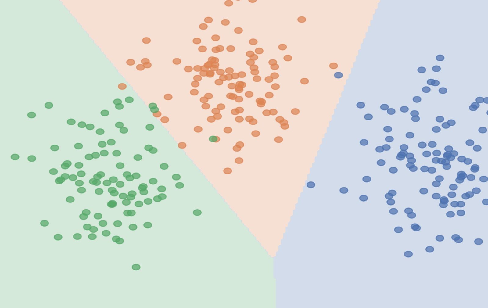
Linear Discriminant Analysis (LDA) in Real-Life: Dimensionality Reduction in a Real-Estate Dataset

Linear Discriminant Analysis (LDA) is a supervised learning technique used to surface the core components, or patterns, in the data.

In this article we’re going to see how LDA works with a real-life example, how it is used to reduce the dimensionality of a dataset and identify class separation boundaries.

···

Linear Discriminant Analysis is a statistical technique, typically applied in the data preparation phase of Machine Learning Classification problems [1]. It’s used to reduce the dimensionality of a dataset, and highlight the characteristics of the data that best ensure the separability of its different classes.

One major application of LDA, for instance, is in image classification[2]. Image classification datasets tend to have thousands of features and LDA is used to reduce the number of features that can be used to properly distinguish between classes, and then run a classification machine learning algorithm on a much smaller feature space.

Linear Discriminant Analysis: the technique

In literature, LDA can also be referred to as Normal Discriminant Analysis or Fisher Linear Discriminant Analysis, the latter being a reference to Ronald A. Fisher, the polymath who developed the criterion LDA aims to maximize.

Fisher’s Criterion: the ratio of between-class and within-class variance [2]

The goal

The idea behind LDA is to take a dataset with high-dimensionality, e.g., a dataset with hundreds or thousands of features, and represent that same dataset with a smaller number of features.

After applying LDA, you don’t necessarily have features, you’ll have different linear discriminants, which still encode the original characteristics of the data.

This latter point is crucial. This technique will reduce the amount of information that is used to describe the original dataset, because originally you had a large amount of features and afterwards you have maybe a handful of discriminant components. However, the characteristics of the original dataset are preserved, meaning, the dataset is just encoded in a much smaller feature space.

It’s almost like you have a super complex music piece, with tons of notes for different instruments and then convert it to MIDI, which is encoded and transmitted in 8-bit bytes. Nevertheless, in the MIDI version you’re still able to distinguish the melody. The bones, i.e., the core characteristics of that music piece are still there, they’re just encoded in a lower-dimensionality space.

Additionally, LDA ensures the different classes in the dataset are as distinguishable as possible, such that you’re able to separate the data points in each class as much as possible.

Assumptions

Before jumping into the mathematical definition, it’s important to mention that LDA must take into account a few assumptions:

1. Data is linearly separable

2. Data follows a Gaussian (Normal) Distribution

3. Shared Covariance matrix across all classes

Data is linearly separable

This is a very strong assumption for this technique, the name gives it away, Linear Discriminant Analysis.

If you attempt to apply LDA to a dataset that is not linearly separable, i.e., the boundaries between the classes in the data are curves and not lines, you may get discriminants, but they may not be the best encoding of the core characteristics of the dataset. LDA is known to fail to properly capture nonlinear relationships and manifold structures in the data[3].

Data follows a Gaussian (Normal) Distribution

This technique assumes that data from each class is drawn from a Gaussian Distribution, i.e., the Normal Distribution[4].

Shared Covariance matrix across all classes

In order to maximize the separability between classes, LDA needs to look at the variance in the data. However, since we’re working with high-dimensionality data, i.e., matrices, instead of scalars, we can’t use the variance as the measure of spread or dispersion. We need to use a covariance matrix.

Succinctly, the covariance matrix describes the amount of spread each feature has, along its diagonal, as well as, the correlation between each pair of features, on the off diagonal.​

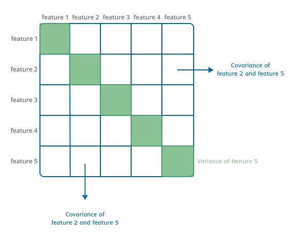
Specifically for LDA, the assumption is there’s a shared variance across all classes, meaning that each within-class covariance matrix is the same across all classes. This is necessary to ensure the pooled, i.e., shared, within-class covariance matrix is an accurate representation of each within class covariances[5].​

Mathematical Definition

Mathematically speaking, Linear Discriminant Analysis identifies the linear combination of features that best discriminate or distinguish between classes in the data[5].

This method approximates the Bayes Classifier [6], which assigns an observation to a class for which the posterior probability, i.e., the probability the observation belongs to a class k, is the greatest.

​Recapping the Bayes Theorem:

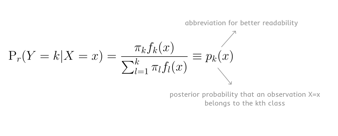
Let’s unpack this. In the formula above we have:

• Y – the label, i.e., the qualitative response variable

• K – total number of classes, i.e., labels, in the data

• k – individual instance of a class in the data

• Pi_k- prior probability that a randomly chosen observation comes from class k

• fk(x) – density function of X for an observation that comes from class k. It’s the probability of X given Y = k , only because we’re working with a qualitative random variable X

Since we’re assuming the data follows a Gaussian Distribution, we can update the general Bayes Theorem formula above and replace the density function placeholder, for the density function of the Gaussian Distribution.​

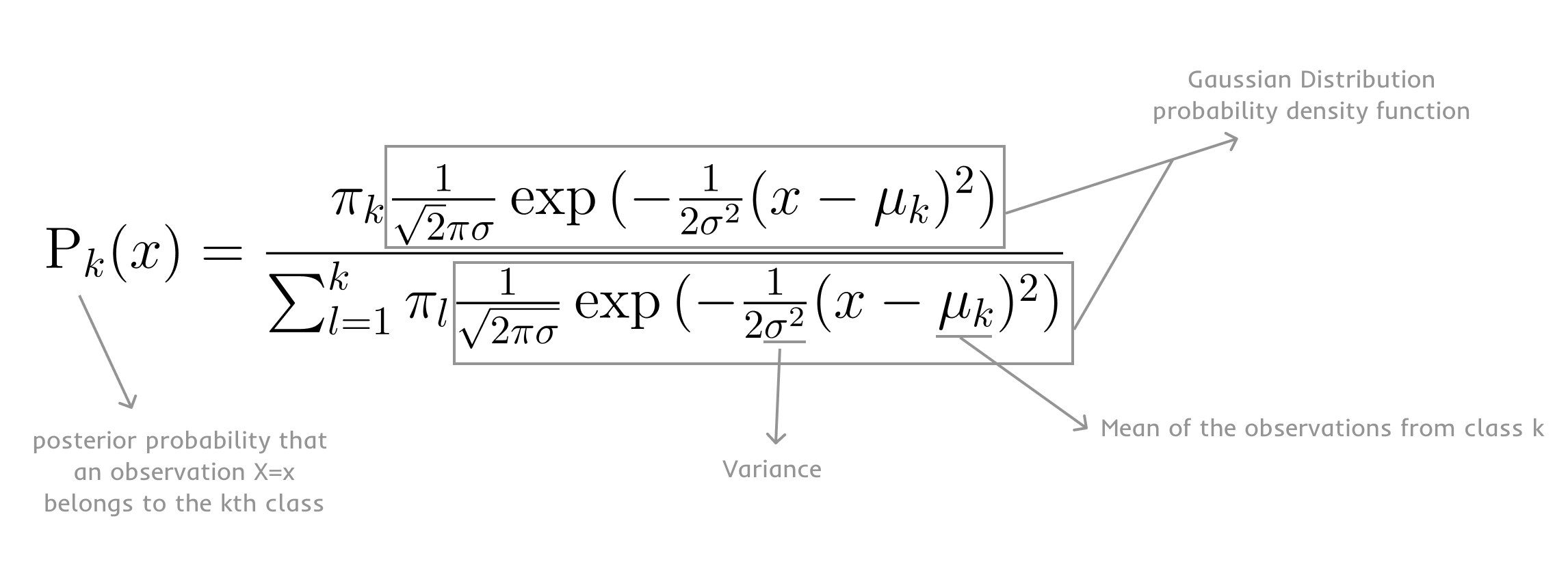
Looking at the formula above, you can tell it is a bit verbose. So, taking the logarithm of the entire formula and doing some algebra, you get a much more concise definition of the posterior probability that an observation X=x belongs to the kth class.

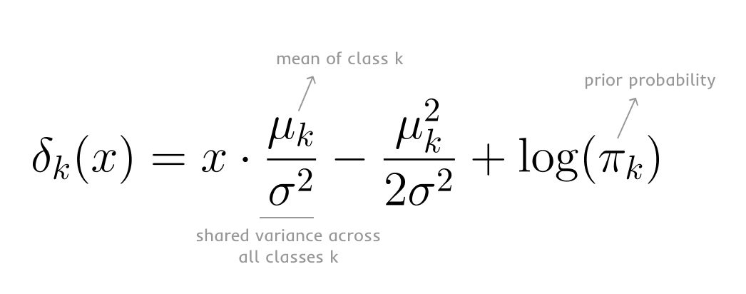
The Bayes Classifier will assign an observation to a class where the quantity above, posterior probability, is the largest.

This sounds very similar to what Linear Discriminant Analysis does!

And that’s the right intuition, because LDA takes the Bayes Classifier and approximates it by explicitly using estimates for:

• Prior probability

• Mean of class k

• Shared covariance across all k classes

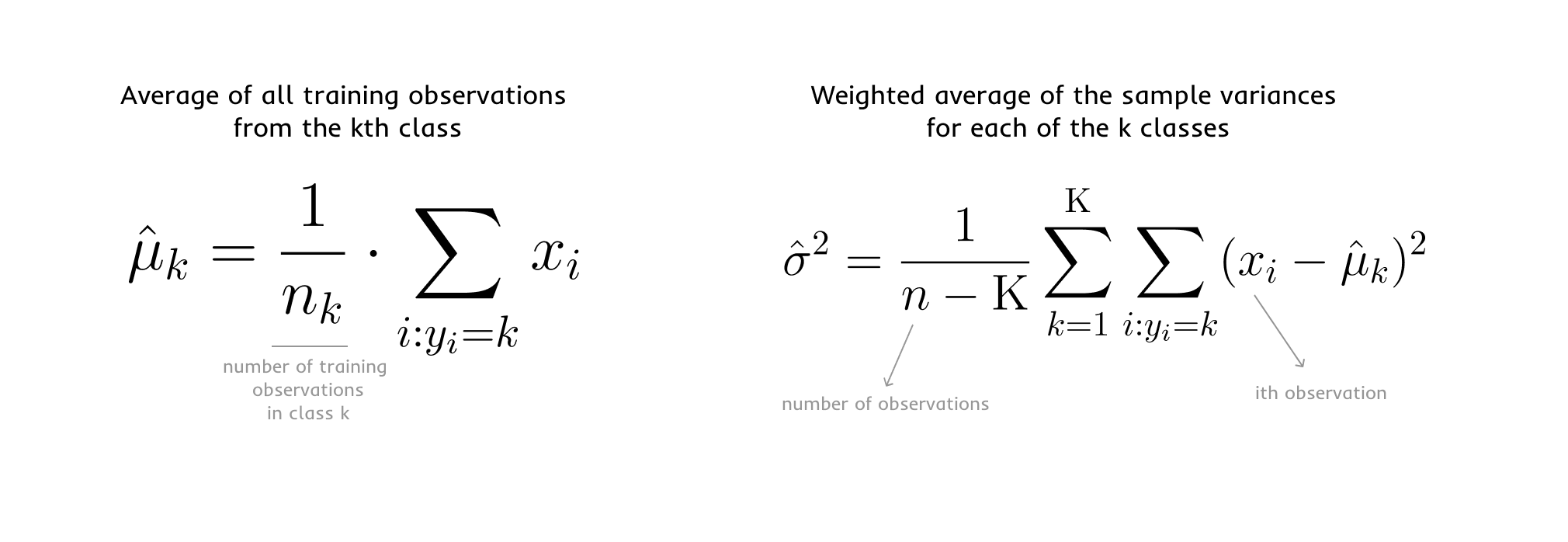
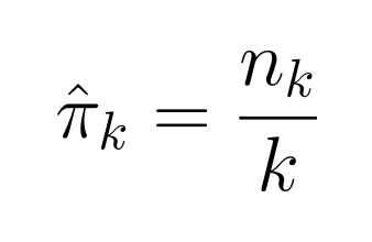
Lastly, if we don’t have information about the true prior probability, we can estimate it based on the proportion of the training observations that belong to class k.

If you’re ever in doubt if you’re dealing with the true quantity or an estimator, note that, in algebra and statistics, the estimators always have a hat (^).​

Putting it all together, after taking into account all the necessary assumptions and the Bayes approximation, the LDA algorithm calculates the discriminant function for each individual data point x of the Gaussian variable X (X=x) and for each class k. It will only assign x to the class for which the discriminant function is the largest:

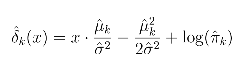
So, in the end, the discriminant function must be a linear function of x.

But this formula above was for the specific case when we only have one predictor, where x is a scalar, i.e., just a number.

In the type of problems LDA is applied to, there are typically hundreds or thousands of predictors, i.e., features. We’re no longer working with scalars, but with matrices. Sometimes very large, sparse matrices.

The Multivariate Gaussian variable X takes the following shape:

Where each data point x is a row vector 1xN, following the Gaussian Distribution, where N is the number of predictors and is greater than 1. When you put all the data training data points together, you have the training dataset, a matrix.

Since we’re working with a Multivariate Gaussian Distribution the probability density function is

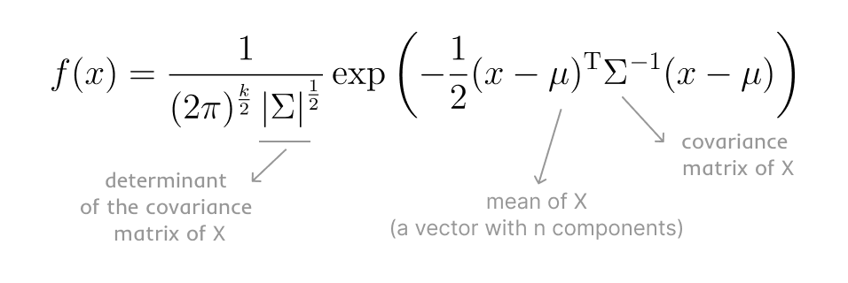
Again, this is a bit verbose. Following the same algebra as before, we can simplify this function a bit and obtain the linear discriminant function for the multivariate case.

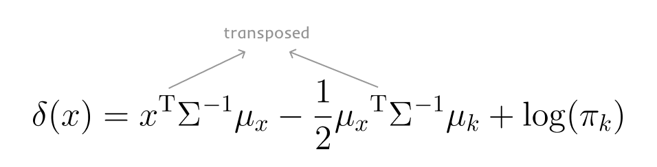
Similarly, the discriminant function still needs to be a linear function of X.

The LDA algorithm calculates the discriminant function for each individual row vector x and for each class k. It will only assign x to the class for which the discriminant function is the largest.

Now, let’s take a step back from all this intricate math.

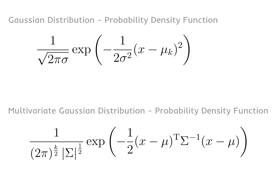
If you compare the Bayes Classifier approximation formula for the single predictor with the one for the multivariate predictor, the one main difference is in the probability density function of the distribution.

The why

Even though this technique is based on a statistical method developed in the 1930s, there are a few reasons why its application is still very relevant today:

• Reduces computational complexity and effort (also saving money)

• Removes redundant features

• Reduces overfitting

• Facilitates visualization interpretability

Reduces computational complexity and effort

Running a Machine Learning algorithm on a dataset with thousands of features can be computationally complex, thus requiring specialized hardware like GPUs or TPUs, may take a long time to run and, as a consequence, may cost lots of money.

As fine-tuned or streamlined algorithms might be, running standard matrix operations, such as multiplication, inversion or eigenvectors and eigenvalues, on a 10×10 matrix tends to be computationally less expensive than running the same operations on a 100×100, 1000×1000 or 10000×10000 matrix.

So, reducing the size of the matrix for computation, granted that the characteristics of the data are preserved, is a huge advantage.​

Removes redundant features

Since this technique aims to minimize the within-class variance, while maximizing the between-class variance [3], it will necessarily give a lower weight to all features that don’t contribute to separate the classes and will drop any features that redundant.

In the end, the algorithm will remove those features that encode the same information as other features that are more relevant to distinguish between different classes.

Reduces overfitting

When we have a dataset with a large number of features, it’s possible the classifier picks up the wrong signals, like noise in the data or correlations that don’t necessarily help distinguish between the different classes. But because those signals are so strong, the classifier can overfit to those signals.

Since LDA reduces the dimensionality of the dataset, keeping the components that best encode the characteristics of the data and, as mentioned above, also removes redundant features, it can help reduce overfitting.

Facilitates visualization interpretability

Linear dimensionality reduction techniques such as LDA tend to preserve data interpretability, because they project the data into discriminant functions that are a linear combination of the original features. Meaning, the linear discriminants represent the axes that best separate the data points into the different classes. This allows for a direct mapping of the feature contributions and for a better understanding of the results [3].

Since the data is projected in a lower-dimensionality space, it’s also possible to better visualize the separation between classes.

Before applying LDA, it might have been hard to plot the data due to the large number of features. Post-LDA, with the data encoded into components that can map to groups of features instead of being 1:1 with each feature, it’s likely you can plot the data in such a way that is possible to easily visualize the separation between classes. ​

Limitations

Like any other technique, this one also has its limitations.

LDA’s main limitations are connected to its assumptions.

With the strong linearity assumption, it is not the best technique for noisy or sparse data and may not provide the most accurate results on classification problems with non-linear decision boundaries or distributions that are not Gaussian[4].

The estimation of the covariance matrix, specifically in high-dimensional data can also pose limitations. When the number of features is relatively large, compared to the number of observations, the covariance matrix can have a high estimation variance and cause performance issues, even when all other assumptions hold [4].

Linear Discriminant Analysis (LDA) vs Principal Component Analysis (PCA)

When thinking about statistical techniques to reduce the dimensionality of a dataset, another very popular technique may come to mind, the Principal Component Analysis.

Although you can find similarities between them, there’s one striking difference. LDA is a supervised method, meaning, it uses the information about the features and the classes/labels associated with each data point when it’s calculating the discriminants, while PCA doesn’t [7]. Given this distinction Linear Discriminant Analysis tends to be a much more robust method for dimensionality reduction [2].

Both techniques are used to reduce the dimensionality of a dataset and, in the end, both produce the axes or the direction vectors that are used to project the original dataset into the reduced dimension space.

The distinction between the two techniques comes in the fact that PCA computes the eigenvectors and ranks them by the associated eigenvalues that have the largest variance, while LDA computes the eigenvectors that best discriminate between classes.

Another difference between PCA and LDA refers to the number of non-zero eigenvectors that can be calculated. In the case of PCA those are tied to the Principal Components and, in LDA, to the Linear Discriminants.

There is a maximum of K-1 Linear Discriminants that can be calculated in LDA, with K being the number of classes[8]. In practice the LDA algorithm calculates all the different eigenvectors, but only K-1 are non-zero.

On the other hand, PCA doesn’t have this limitation.

In short, we have that PCA, being an unsupervised method, produces the Principal Components, i.e., the direction vectors, that best describe the original dataset. On the other hand LDA, being a supervised method, produces the Linear Discriminants that best discriminate, or separate the data, among the different classes [7].

LDA real-life example

If you’ve read my article on Principal Component Analysis, you’ll be familiar with this example.​

Your friend Maggie is a real-estate agent and wants some hard data about what really distinguishes the properties she has sold. So she asks you, her Data Scientist friend, to help with this task.​

As always, the first step is to take a look at the dataset at hand, using the following Python code.

import pandas as pd##### Data Preparation##### Importing the dataset and loading it into a dataframedataset_df = pd.read_csv("../datasets/dataset_labeled.csv")print(dataset_df.head())

The output is a nice peek at the data.

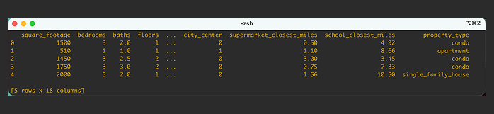
At this point you’re just getting familiar with the different features, such as:

• square_footage – square footage for the property

• bedrooms – number of bedrooms in the property

• baths – number of baths in the property

• …

And with the dataset label, property_type. There are three possible values for the dataset label: apartment, condo, single_family_house.​

With so many features, it’s really hard to pinpoint or even visualize how the data is spread across the different types of properties.

That’s when you remember you can use Linear Discriminant Analysis to both visualize how the data about the different property looks like, meaning, are the data points about condos all clustered together and far apart from the data points for single family houses or apartments?

At the same time, you’ll be able to get more information about what distinguishes the different types of properties in the dataset.

You immediately think about using the LinearDiscriminantAnalysis function from ScikitLearn, and you start putting your code together.

import pandas as pdfrom sklearn.discriminant_analysis import LinearDiscriminantAnalysisfrom sklearn.preprocessing import StandardScaler##### Data Preparation##### Importing the dataset and loading it into a dataframedataset_df = pd.read_csv("dataset.csv")# Setting our X (features) and y (labels)y = dataset_df["property_type"]X = dataset_df.drop(columns=["property_type"]).to_numpy()feature_names = dataset_df.drop(columns=["property_type"]).columnstarget_names = y.unique()# Normalize the features # so they're all on the same scale before fitting LDA# This will help with the visualization of the covariance matrix# Therefore all values are in the same scale# Normalization will not affect the LDA processX = StandardScaler().fit_transform(X)##### Applying the LDA function##### Customizing the following parameters#   solver='eigen':: using eigenvalue decomposition#   covariance_estimator:: is left with the default value of None, since we're going to use the covariance matrix#   n_components = 2: setting the number of components to 2 #       The number of components must be, at most, be equal to the number of labels minus 1# Leaving the shrinkage factor as default = None, since we're going to use the covariance estimatorclf = LinearDiscriminantAnalysis(solver='eigen', n_components=2)# Fits the LDA model and applies the function transform()# to help maximize separation between classesX_lda = clf.fit(X, y).transform(X)###### Stats about the Linear Discriminant Analysis##### Calculating the Accuracy of the training data# in this case, since we're not interested in predicting classes,# the entire dataset is used in this functionprint("Training dataset accuracy %f" % clf.score(X, y))

​You have your data imported from CSV into a Pandas DataFrame for manipulation. Then separate between the features (X) and the labels (y), which is going to be used later in the fitting of the classifier.

One thing you also have in mind is to visualize the Covariance Matrix of the dataset, so you can see the covariance between pairs of features. Since you know upfront you want to do this and, acknowledging lots of features are in different scales, you first normalize the feature matrix X.

Notice that at the top, there was no need to split the data into training and testing. Maggie’s questions are not tied to predicting the type of property a new, never seen before, data point corresponds to. So you don’t actually need to split the data, you use it all to fit the LinearDiscriminantAnalysis function.

With the LinearDiscriminantAnalysis applied to the dataset, one of the things you check is the training accuracy of ~98%.

In the end, the data normalization won’t make any difference when you fit the LinearDiscriminantAnalysis. It will just make it easier to visualize the Covariance Matrix with the following code.

#additional importsimport seaborn as snsimport matplotlib.pyplot as pltdef plot_covariance_matrix(clf, feature_names):    """Plot the pooled within-class covariance matrix as a heatmap.    Args:        clf: Fitted LinearDiscriminantAnalysis classifier, used for its covariance_ attribute.        feature_names: Names of the original features, used to label the heatmap axes.    """    plt.figure(figsize=(20, 10))    sns.heatmap(clf.covariance_, cmap="viridis_r", linewidths=.7, annot=True, fmt='.2f',                xticklabels=feature_names, yticklabels=feature_names)    plt.title("LDA: Pooled Within-Class Covariance Matrix")    plt.tight_layout()    plt.savefig("plot_covariance_matrix.pdf")plot_covariance_matrix(clf, feature_names)

The output is this colorful matrix with the variance or spread of each feature on the diagonal and the correlation between features on the on the off diagonal.

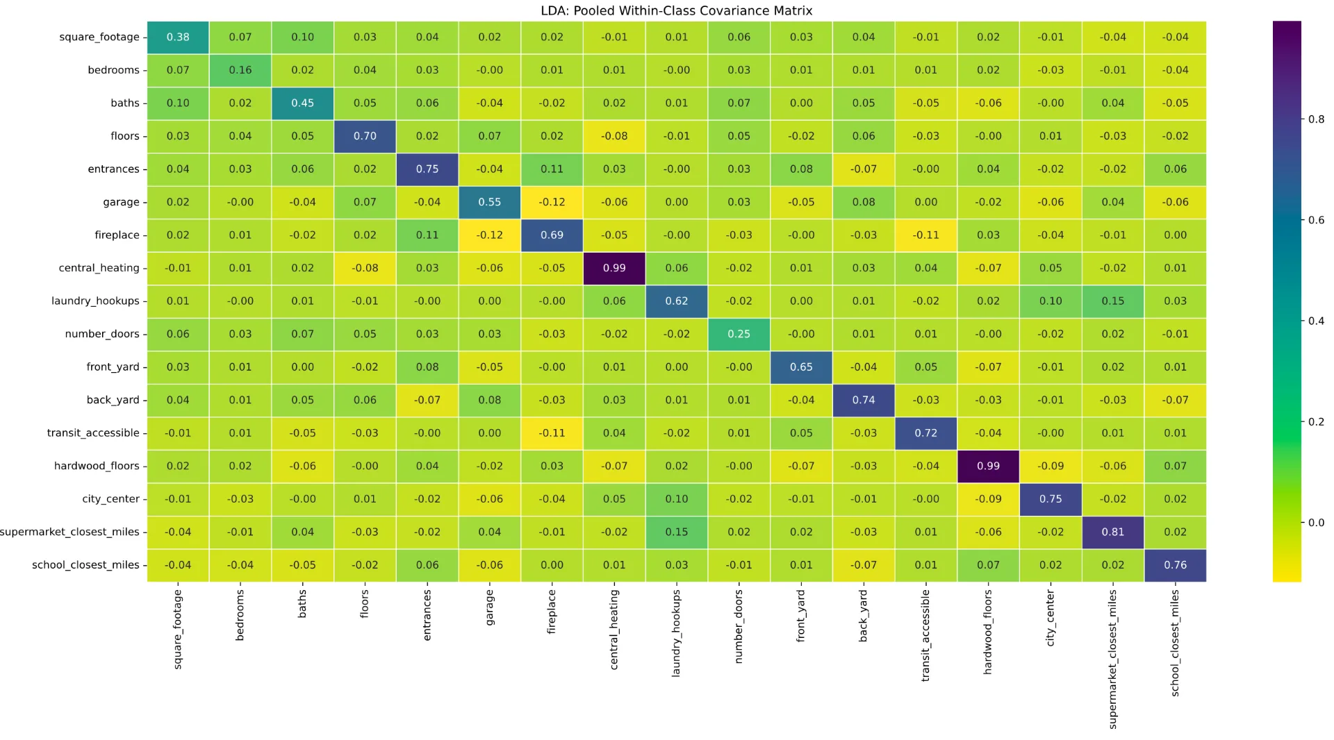
This is great! Doesn’t necessarily answer Maggie’s question, but it’s good to check, from a data exploration perspective. Especially to spot check features that are highly correlated with each other.

Back to Maggie’s questions.

First she was interested in understanding if data points about condos all clustered together and far apart from the data points for single family houses or apartments.

This is something we can try to visualize after reducing the dimensionality of the dataset.

You already fit the LinearDiscriminant, so now you need to plot the data points in the two Linear Discriminants and color them based on their corresponding label.

So, you add a new function to your codebase.

#Colors for each property_type, kept consistent across all plotsproperty_colors = {    "apartment": "#4C72B0",    "condo": "#DD8452",    "single_family_house": "#55A868",}def plot_components(X_lda, y, target_names):    """Plot the LDA-transformed data on LD1 vs LD2, colored by property type.    Args:        X_lda: LDA-transformed feature matrix, with LD1 and LD2 as the first two columns.        y: Series of property_type labels aligned with the rows of X_lda.        target_names: Array of unique property_type labels, used to plot each class separately.    """    plt.figure(figsize=(10, 7))    for target_name in target_names:        # builds an array (mask) with the same length as the label array y        mask = y == target_name        # the mask is used to separately plot the points belonging to each class        plt.scatter(X_lda[mask, 0], X_lda[mask, 1], label=target_name,                    color=property_colors[target_name], alpha=0.7)    plt.xlabel("LD1")    plt.ylabel("LD2")    plt.title("LDA: Property Type Separation by LDA Component")    plt.legend(loc="best")    plt.savefig("plot_lda_components.pdf")plot_components(X_lda, y, target_names)

The output is this plot, where you can see there’s a more marked separation between apartments and single family houses and classification-wise, in this dataset a condo is closer to a single family house than to an apartment.

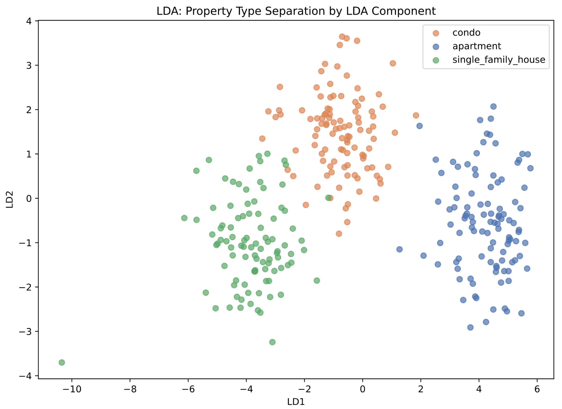
This plot is really great because, you started off with a dataset with 17 features and 3 classes. As you can imagine it would be very difficult to visualize the layout of the data and the separation between classes based on 17 features. You could plot each pair of features against each other, but it would never be a full picture.

With LDA, you reduced the dimensionality to 2 Linear Discriminants which, in this case, is the maximum number of components you could have. The maximum number of Linear Discriminants is the minimum between the number of features and the number of classes minus one. In this case, number of classes minus one wins, and you picked n_components = 2.

This is very handy, because a 2D plot is something most people are used to interpret, and will help Maggie literally get a better picture of the separation between the different types of properties.

But you’re a data scientist and sometimes like to show how you can make your visualizations shine. In this case, you want to do this by adding the decision boundary that separates each class. It will elevate your visualization and show Maggie you’re really up to the task!

So you create a new function, similar as the one for the LinearDiscriminant plot, but where you draw a mesh where you’ll draw the points that make up each decision boundary.

#additional importfrom matplotlib.colors import ListedColormapdef plot_components_with_approx_boundary(X_lda, y):    """Plot LD1 vs LD2 with an approximate decision boundary, colored by property type.    The boundary is "approximate" because it comes from a classifier fit directly    on the 2D LD1/LD2 projection, not the original feature space.    Args:        X_lda: LDA-transformed feature matrix, with LD1 and LD2 as the first two columns.        y: Series of property_type labels aligned with the rows of X_lda.    """    boundary_clf = LinearDiscriminantAnalysis()    boundary_clf.fit(X_lda, y)    # Setting the boundaries of the mesh (x/y coordinate) grid we're going to use to "draw" the    # approximate decision boundary    x_min, x_max = X_lda[:, 0].min() - 1, X_lda[:, 0].max() + 1    y_min, y_max = X_lda[:, 1].min() - 1, X_lda[:, 1].max() + 1    # Building the mesh grid    xx, yy = np.meshgrid(np.linspace(x_min, x_max, 300), np.linspace(y_min, y_max, 300))    # Reshaping the data in order to predict the labels for each point in the    # decision boundary grid    # 1. the function ravel flattens the 2D arrays into 1D    # 2. function np.c_ stacks those arrays in the columns of a 2D array,     # 3. run the predict function    Z = boundary_clf.predict(np.c_[xx.ravel(), yy.ravel()])    Z = pd.Categorical(Z, categories=target_names).codes.reshape(xx.shape)    # Creating the color map, i.e., assigning a color for each label    boundary_cmap = ListedColormap([property_colors[name] for name in target_names])    plt.figure(figsize=(10, 7))    # Draws the filled contour lines     plt.contourf(xx, yy, Z, alpha=0.25, cmap=boundary_cmap)    # Draws each point for each component, i.e., the LDA-transformed data    for target_name in target_names:        # builds an array (mask) with the same length as the label array y        mask = y == target_name        # the mask is used to separately plot the points belonging to each class        plt.scatter(X_lda[mask, 0], X_lda[mask, 1], label=target_name,                    color=property_colors[target_name], alpha=0.7)    plt.xlabel("LD1")    plt.ylabel("LD2")    plt.title("LDA: Property Type Separation with Approximate Decision Boundary")    plt.legend(loc="best")    plt.savefig("plot_lda_components_approx_boundary.pdf")plot_components_with_approx_boundary(X_lda, y)

This really pushes the previous visualization to another level!

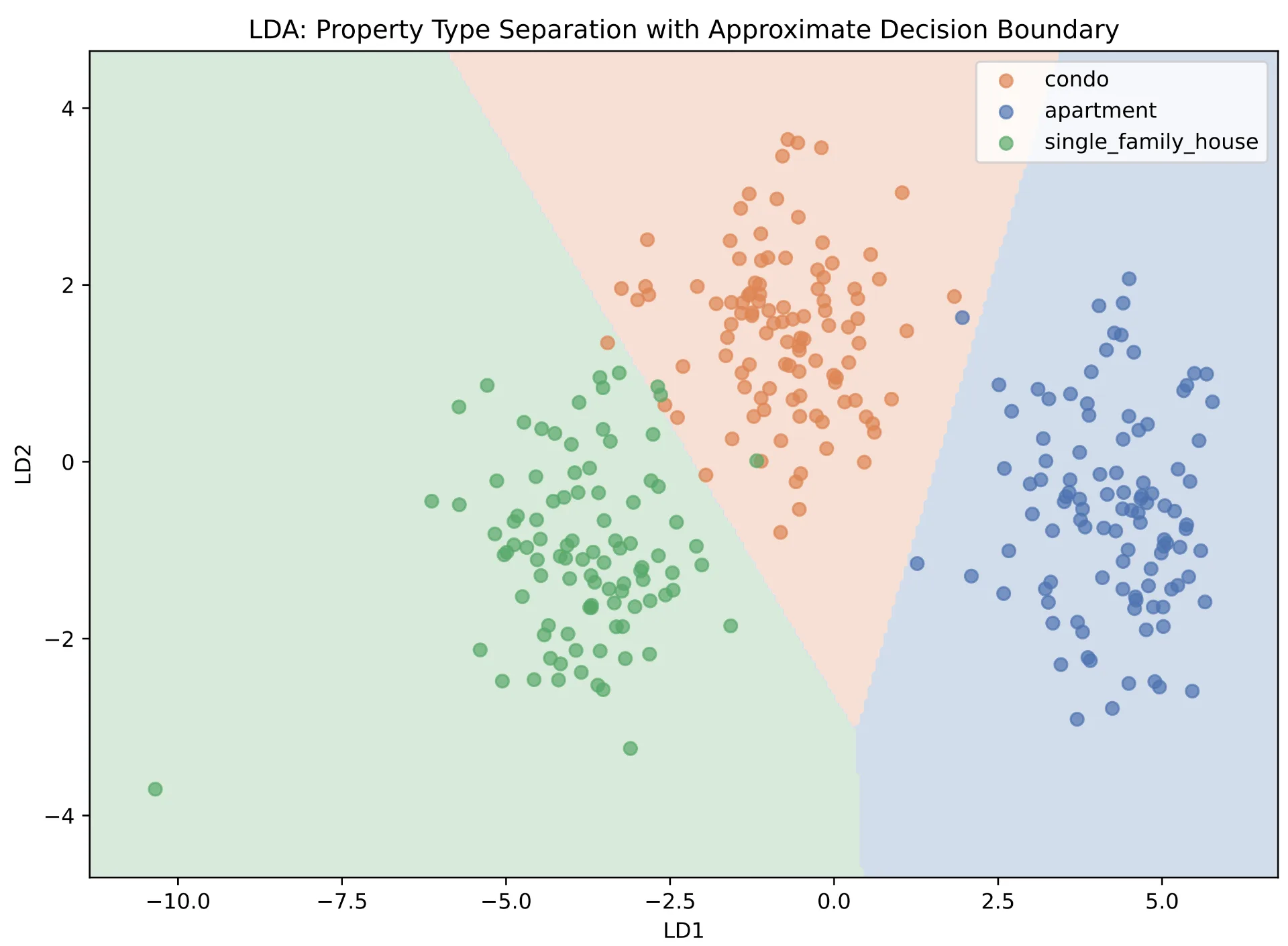
The decision boundaries you’ve drawn are technically approximate decision boundaries. The true decision boundaries come from the original dataset, whereas these were drawn based on the data in the LinearDiscriminant. In practice, they are very close to the true decision boundaries since the Linear Discriminants still encode the main characteristics of the data. However, it’s important to make this distinction.

Now, onto Maggie’s last question: What distinguishes the different types of properties in the dataset?

In order to answer this question you need to turn to the dataset features and see what they can tell you about what distinguishes each class.

So you start looking for ways to get to information about the feature contribution. You gladly remember applying the parameter solver=’eigen’ in the LinearDiscriminantAnalysis function, it means the function using eigenvector decomposition to find the linear discriminants that indicate class separation.

That means you have access to the attribute scalings of the LinearDiscriminantAnalysis function from ScikitLearn and inspect how much each feature contributes to each LinearDiscriminant

By default, scalings will output all the possible eigenvectors, across all features. In this case, you’ll have one eigenvector for each of 17 features in the dataset.

However, you set n_component = 2 in the LinearDiscriminantAnalysis function, those are the only Linear Discriminants that are going to be used to project the data into a lower-dimensionality, i.e., from the 17 features to 2 Linear Discriminants which encode the core information of those features.

In order to output only the two Linear Discriminants, instead of all possible eigenvectors, you just need to truncate the scalings in the plot_class_separation_features.

This way the output is restricted to just the two linear discriminants.

def plot_class_separation_features(clf, feature_names):    """Plot a heatmap ranking the original features by their contribution to class separation.    Uses clf.scalings_, the eigenvectors LDA assigns to each original feature per    component, to show which features carry the most weight for LD1, LD2, etc.    Darker blue means a larger contribution to that component's class separation.    Args:        clf: Fitted LinearDiscriminantAnalysis classifier, used for its scalings_ attribute.        feature_names: Names of the original features, used to label the heatmap rows.    """    # scalings_ holds the full eigenvector basis (n_features columns), but only the    # first n_components are actually used by transform() for class separation    scalings = clf.scalings_[:, :clf.n_components]    component_names = [f"LD{i + 1}" for i in range(scalings.shape[1])]    weights = pd.DataFrame(np.abs(scalings), index=feature_names, columns=component_names)    weights = weights.sort_values(by="LD1", ascending=False)    plt.figure(figsize=(7, 8))    sns.heatmap(weights, cmap="Blues", linewidths=.7, annot=True, fmt='.2f')    plt.title("LDA: Feature Contribution to Class Separation")    plt.tight_layout()    plt.savefig("plot_class_separation_features.pdf")# Ranks the original features by how much they contribute to class separationplot_class_separation_features(clf, feature_names)

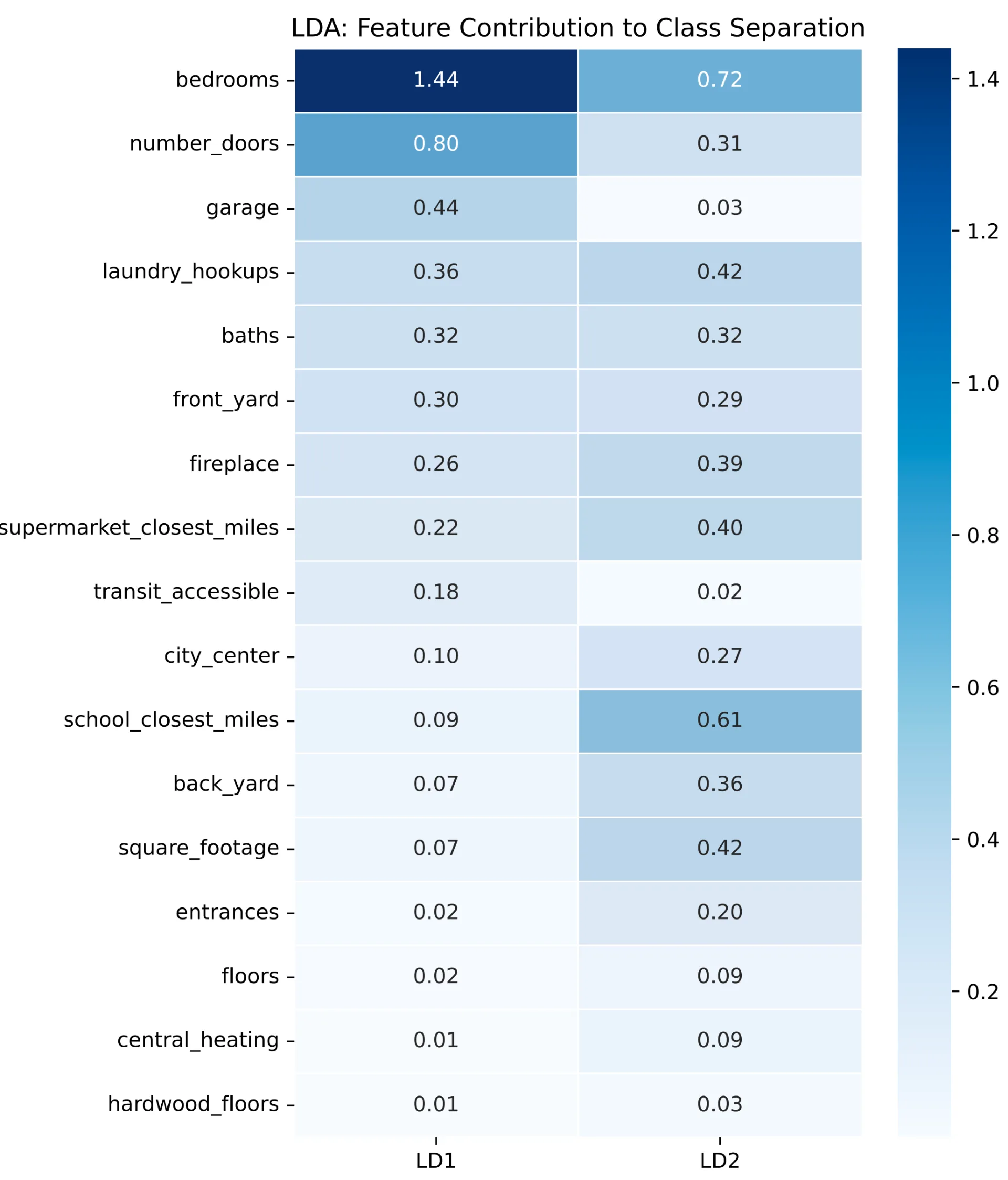
Something that jumps right away is the scale. Indeed you can see that bedrooms is the feature that, individually, contributes the most to each linear discriminant. However, it’s a bit hard to interpret because this is not a 0-100% scale. Instead these values are relative to each other and are based on the raw values of the eigenvector decomposition.

To better understand how each feature contributes to each Linear Discriminant, you decide to normalize the values in each linear discriminant column. The total contribution of all features towards each individual linear discriminant will total to 100%.

To keep things separate, you create a new function, in all similar to the one you just created, but it normalizes the values of the output of scalings.

def plot_class_separation_features(clf, feature_names):    """Plot a heatmap ranking the original features by their contribution to class separation.    Uses clf.scalings_, the eigenvectors LDA assigns to each original feature per    component, to show which features carry the most weight for LD1, LD2, etc.    Darker blue means a larger contribution to that component's class separation.    Args:        clf: Fitted LinearDiscriminantAnalysis classifier, used for its scalings_ attribute.        feature_names: Names of the original features, used to label the heatmap rows.    """    # scalings_ holds the full eigenvector basis (n_features columns), but only the    # first n_components are actually used by transform() for class separation    scalings = clf.scalings_[:, :clf.n_components]    component_names = [f"LD{i + 1}" for i in range(scalings.shape[1])]    weights = pd.DataFrame(np.abs(scalings), index=feature_names, columns=component_names)    weights = weights.sort_values(by="LD1", ascending=False)    plt.figure(figsize=(7, 8))    sns.heatmap(weights, cmap="Blues", linewidths=.7, annot=True, fmt='.2f')    plt.title("LDA: Feature Contribution to Class Separation")    plt.tight_layout()    plt.savefig("plot_class_separation_features.pdf")# Ranks the original features by how much they contribute to class separation. Normalized so each component's weights sum to 1plot_class_separation_features_normalized(clf, feature_names)

In the end, the rankings of how much each feature contributes to each linear discriminant is the same but, making it such that the sum of all contributions within each linear discriminant sum to 100% is a reassuring and definitely much easier to interpret.

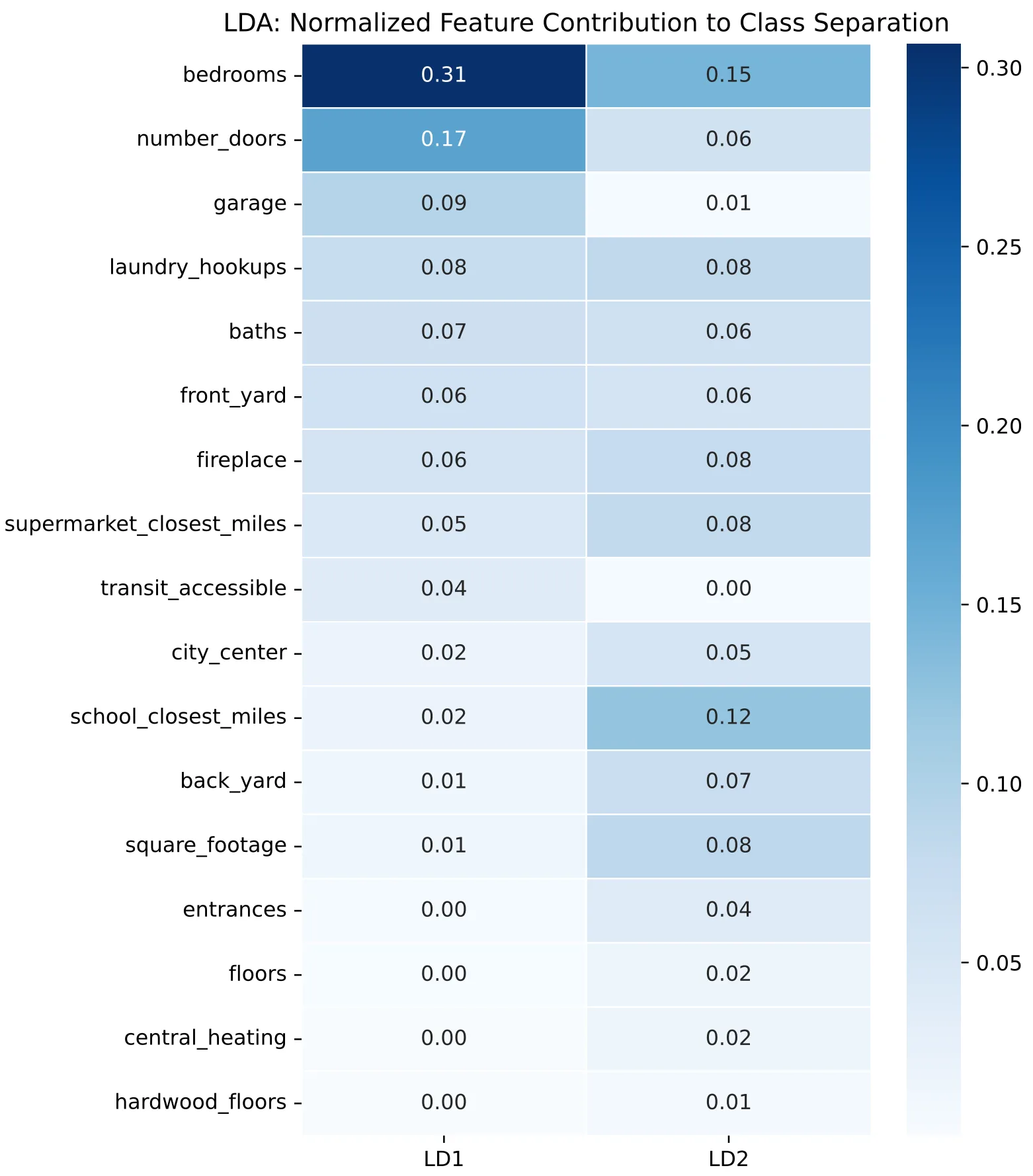
Initially, for the second linear discriminant, the first and second highest feature contributions were for:

• bedrooms = 0.72

• school_closest_miles = 0.61

Which seems like there was a slightly significant difference between them.

Post-normalization you can see that, towards the second linear discriminant, the contribution of bedrooms is 0.15 compared to 0.12 for school_closest_miles. Doesn’t seem like such a wide gap as before.

Unfortunately this technique doesn’t allow you to compare feature importance across Linear Discriminants, but there’s still a way to piece together different information the Linear Discriminant Analysis provides and answer Maggie’s question: What distinguishes the different types of properties in the dataset?

One you can check to answer this question is the Explained Variance, since it provides the ratio of how much of the separation between classes is explained by each component. You just need to output the explained_variance_ratio_ attribute from the LinearDiscriminantAnalysis classifier.

# The explained variance ratio outputs a list with the percentage of variance# (separation between classes) explained by each component. The list is in component orderprint("Explained Variance Ratio for each component %f", clf.explained_variance_ratio_)

You were already expecting that the first Linear Discriminant would be the one that explains the highest amount of variation, since the first one is always the one with the higherst eigenvalue. And you can see the huge delta between the explained variability from the first to the second Linear Discriminants.

The first Linear Discriminant explains approximately 90% of the separation between classes!

With this information along with the data from feature contribution towards the first Linear Discriminant, it’s not 100% bullet proof, but you can intuit which features will tend to weigh more towards the separation between classes.

You can intuit that bedrooms, garage and laundry_hookups are the features that contribute the most to the separation between classes, since they are the features with the highest importance towards the first Linear Discriminant and we know that the first Linear Discriminant contributes approximately 90% to the distinction between classes.

With the decision boundary plot and this information about feature contribution, you can get back to Maggie and share the insights about the properties she sold!

···

Hope you enjoyed learning about Linear Discriminant Analysis. It’s a very interesting and powerful statistical technique, used as a data preparation step for Classification problems in Machine Learning.

Thanks for reading!

References

1. https://sebastianraschka.com/Articles/2014_python_lda.html

2. C. Gambella, B. Ghaddar, and J. Naoum-Sawaya, “Optimization problems for machine learning: A survey,” European Journal of Operational Research, vol. 290, no. 3, pp. 807–828, May 2021.

3. Wani AA. “Comprehensive review of dimensionality reduction algorithms: challenges, limitations, and innovative solutions,” PeerJ Comput. Sci., vol. 11, p. e3025, 2025, doi: 10.7717/peerj-cs.3025.

4. C. Shen and Y. Dong, “Linear Discriminant Analysis with Gradient Optimization,” arXiv preprint arXiv:2506.06845, 2026.

5. S. Gardner-Lubbe, “Linear discriminant analysis for multiple functional data analysis,” J. Appl. Stat., vol. 48, no. 11, pp. 1917–1933, 2021, doi: 10.1080/02664763.2020.1780569.

6. T. Hastie, R. Tibshirani, and J. Friedman, The Elements of Statistical Learning: Data Mining, Inference, and Prediction, 2nd ed. New York, NY, USA: Springer, 2009

7. A. M. Martinez and A. C. Kak, “PCA versus LDA,” IEEE Transactions on Pattern Analysis and Machine Intelligence, vol. 23, no. 2, pp. 228-233, Feb. 2001, doi: 10.1109/34.908974

8. C. M. Bishop, Pattern Recognition and Machine Learning. New York, NY, USA: Springer, 2006