The Symmetry That Breaks Neural Network Averaging

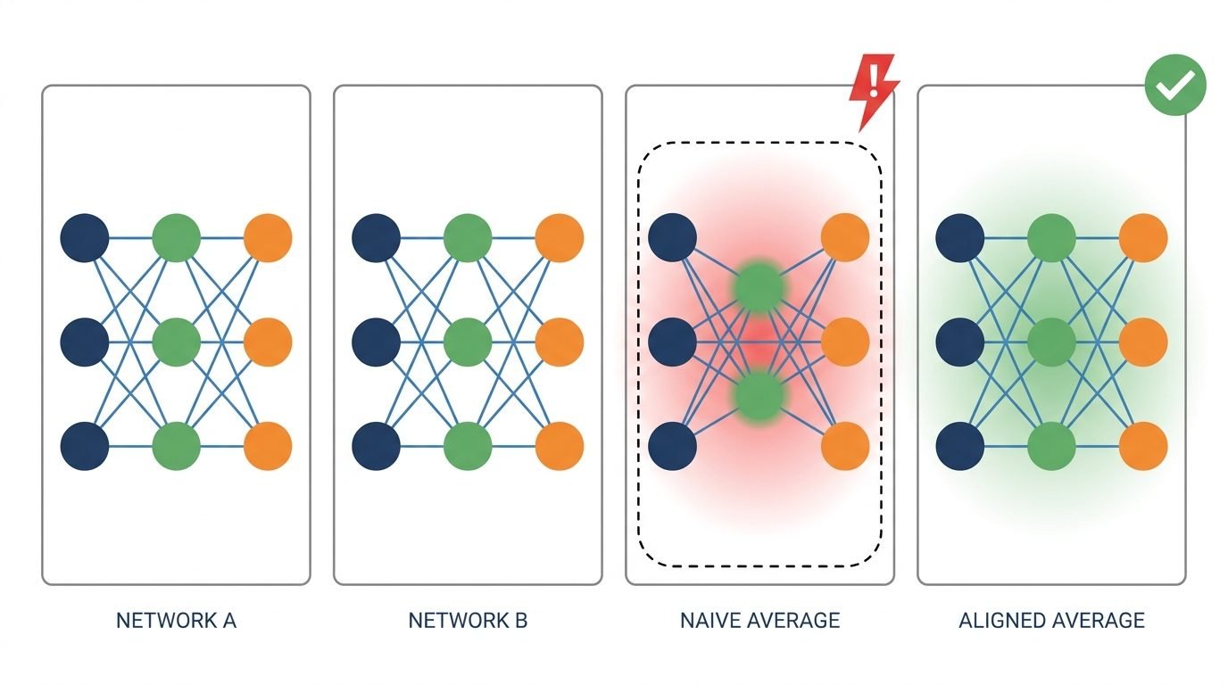
If you have ever tried neural network weight averaging by training the same neural network architecture twice on the same data, changing nothing but the random seed, you have probably assumed the two results were basically interchangeable. Both runs converge. Both reach the same loss. So you average the two weight vectors, expecting something at least as good as either one alone.

The average is worse. Often much worse.

There were no problems during the training process; this is a structural feature of neural networks and can be directly deduced from a property known as permutation symmetry. The same principle also accounts for why model merging succeeds when it does and fails when it fails, a question which, in 2026, is at the heart of practical LLM engineering, whether one is dealing with model soups or federated averaging.

Here is a way to hold the idea before the notation arrives. Think of two trained networks as two spreadsheets describing the same report, except the columns are in a different order. Model A’s “column 3” might hold what Model B calls “column 7.” Both spreadsheets are correct. Both add up to the same totals. But average them cell by cell without first lining the columns up, and you’re averaging revenue with headcount. That’s what naive weight averaging does to a neural network, and it’s worth keeping that image in mind through everything below.

Most introductions to neural networks stay in function space: what the network computes, how an activation function bends a line into a curve. This article stays in parameter space: what the set of good solutions actually looks like, and what that geometry costs you.

Why Neural Networks Are Non-Convex: Adaptive Basis Functions and Permutation Symmetry

Many classic machine learning models have the form:

whereϕ(x)=[ϕ1(x),…,ϕm(x)]⊤ is a set of basis functions, and a is a coefficient vector. Polynomial regression usesϕℓ(x)=xℓ−1. Kernel ridge regression takes an implicit, effectively infinite basis defined by the kernel k(x,x′)=∑ℓλℓψℓ(x)ψℓ(x′)

In both cases, we are only learning the coefficients a, and the loss is a convex quadratic. One minimum, closed-form solution, no random seeds.

A neural network changes one thing: it makes the basis functions themselves learnable. Each neuron is an adaptive basis function, and the network learns both the basis and the coefficients at the same time by minimizing the same kind of squared-error loss:

That is the whole idea. A neuron is an adaptive basis function. We no longer have to guess which features matter. The network fits the features and the coefficients at the same time by minimizing the function shown below:

This is the core trade-off. Non-convexity is not an accident of ReLU activation. It is the price of adaptivity. Fix the basis, and we get convexity. Learn the basis, and we lose it. There is no third option.

It also explains where the “column order” problem comes from. Polynomial regression’s columns are fixed by convention — x, x², x³, in that order, agreed on in advance. A neural network’s columns are learned along with everything else, which means there’s no agreed-upon order for them to land in. That missing convention is the entire source of permutation symmetry.

Where the non-convexity comes from: Permutation Symmetry

Consider a two-neuron network with one input and ReLU activations:

f(x)=ReLU(x−w1)+ReLU(x−w2)

The loss function is symmetric: swapping w1 and w2 gives exactly the same function, and therefore the same loss. So if (w1,w2) is a global minimum, then (w2,w1) is also a global minimum.

Now, what happens at the midpoint of these two minimizers? By symmetry, the midpoint is ((w₁+w₂)/2, (w₁+w₂)/2) i.e., both neurons have the same parameters. A network with two identical neurons has the expressive power of one neuron, not two. Unless one of the original neurons was doing nothing, the midpoint cannot be optimal.

That’s the whole story. The loss landscape isn’t just bumpy; it contains many exact copies of the same basin, separated by barriers. For a hidden layer with m units, there are m! equivalent orderings. A 512-unit layer gives roughly 512!≈10^1166 copies of every solution per layer. That is 512! different ways to shuffle the same set of columns, each one an equally valid spreadsheet of the same report.

A Simple Two-Neuron Example of Weight Averaging Failure

Two neurons and one input give a landscape we can plot. Take

and generate 200 points from ground truth w = (2,6)with Gaussian noise (σ=0.3).

import numpy as nprng = np.random.default_rng(11)relu = lambda t: np.maximum(0.0, t)x = rng.uniform(0, 10, size=200)y = relu(x - 2) + relu(x - 6) + rng.normal(0, 0.3, size=200)def loss(w1, w2):    pred = relu(x[:, None] - w1) + relu(x[:, None] - w2)    return np.mean((y[:, None] - pred) ** 2, axis=0)

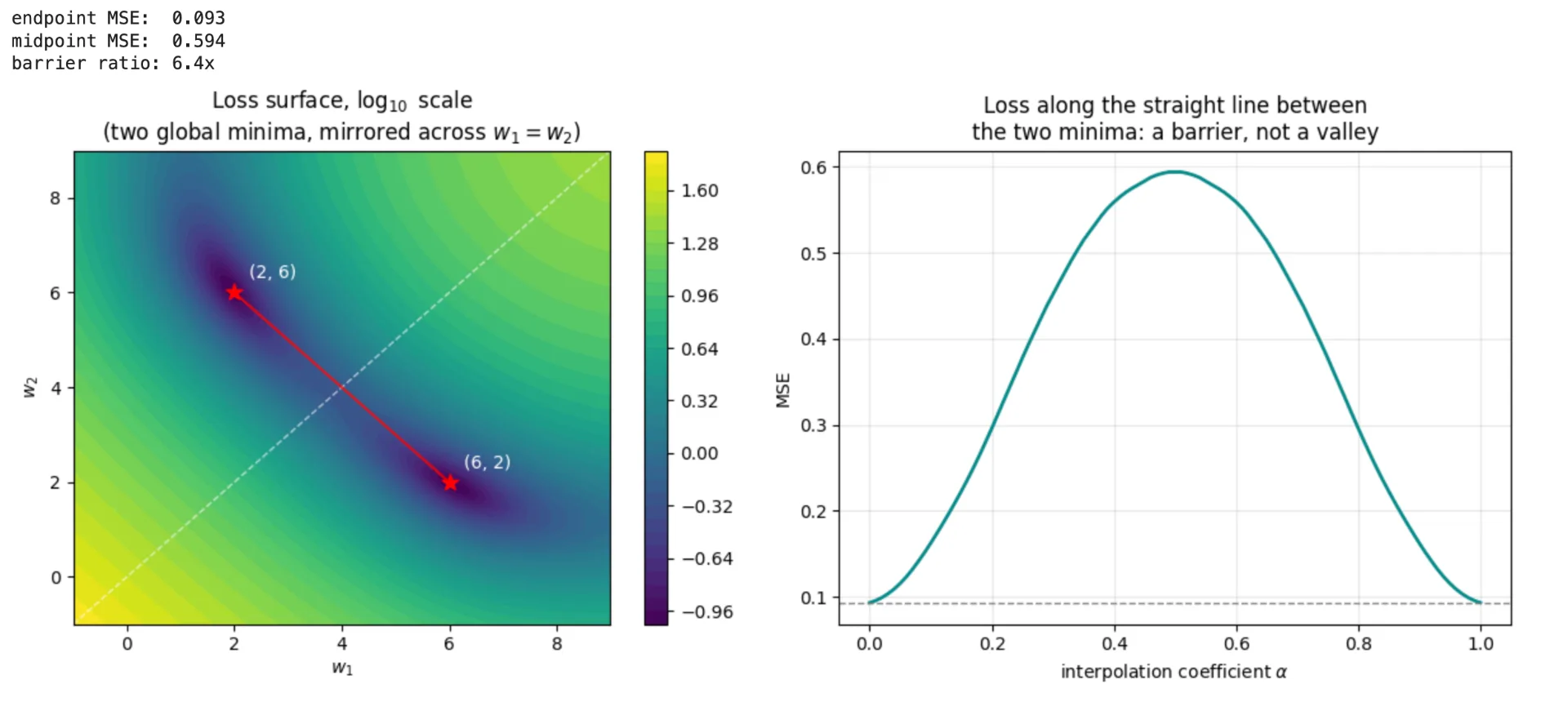
The minima come in pairs. (2, 6) and (6, 2) both sit at MSE 0.093. The surface is exactly symmetric about the diagonal, because the diagonal is the fixed set of the swap.

The straight path between them climbs. The midpoint (4, 4) has MSE 0.594 — 6.4× the endpoint loss. This is a barrier, the same quantity measured in the linear mode connectivity literature, visible here in two dimensions.

Which minimum we land in is a coin flip. Running gradient descent from 40 random initializations, 47% converged to the (2, 6) ordering and 53% to (6, 2). In this example, the seed picks the basin; nothing else does.

Now the merge. Train two models from different starts:

The naive average is 6.5× worse than either input. Permute B’s neurons first; reorder its columns to match A’s, and the average snaps back to a perfect model. Nothing about what B computes changed. Only the labels did.

The same picture at ResNet scale

Entezari et al. (2021) conjectured that most SGD solutions land in the same basin once you quotient out permutation symmetry. Ainsworth, Hayase and Srinivasa (2022) built algorithms to find the aligning permutation and tested it: they argue neural network loss landscapes often contain nearly a single basin after accounting for all possible permutation symmetries of hidden units, and demonstrate near zero-barrier linear mode connectivity between independently trained ResNet models on CIFAR-10. Two networks trained from scratch, independently, merged into one with no loss penalty — after relabelling the units of one.

The caveats matter, and the authors state them. Linear mode connectivity was not observed for narrow models; increasing width progressively drove loss barriers to zero, suggesting the phenomenon requires sufficient capacity. They also conjecture that permutation symmetry is a necessary but incomplete account of the invariances at play. Jordan et al. (2023) showed that, in practice, a further correction to repair activation statistics after interpolation is often needed.

Five Practical Consequences for Model Merging and Weight Averaging

Here are five practical rules that fall directly out of this geometry:

1. Model soups need a common ancestor: Since checkpoints that are fine-tuned from the same pre-trained model remain within the same basin, weight averaging works well in such cases. However, if the various fine-tunings use very different learning rates or regularisation, they might end up in different basins, and the averaging will then fail. It is necessary to check the interpolation curve before averaging.

2. Merging unrelated models requires alignment first: Tools like Git Re-Basin align models modulo permutation symmetries, and REPAIR corrects activation statistics after interpolation. These steps are now standard before task arithmetic or other merging methods.

3. Weight-space distance is not a similarity metric: Since two networks which are functionally identical can be very distant in terms of ℓ2 distance, in particular when continuous symmetries such as rescaling are taken into account, as the labels assigned to neurons are arbitrary. When you are tracking drift or comparing models, you should use representation similarity metrics such as CKA or output agreement on a held-out set instead.

4. Ensemble in function space, not parameter space: Averaging predictions is symmetry-invariant by construction. Averaging weights is not. This is why deep ensembles often outperform weight-averaged models when models are trained independently.

5. Bayesian posteriors over weights are inherently multimodal: A posterior over the weights of an m-unit layer has at least m! identical modes. Mean-field variational inference fits a single Gaussian to this multimodal landscape, which is one reason it underestimates uncertainty. Deep ensembles work partly because independent runs sample different symmetry-equivalent modes.

Permutations are not the only symmetry

It’s important to be aware of this point before you go overapplying the idea. ReLU networks also have a positive-rescaling symmetry: scale a neuron’s incoming weights (and its bias, if it has one) by a positive constant c, and its outgoing weight by 1/c — the function is unchanged, because ReLU is positively homogeneous, ReLU(cz) = c·ReLU(z) for c > 0 (in the case of networks that have no biases). This is similar to a spreadsheet in which one column is measured in dollars, and another paired column in cents i.e., different units but the same information, and no rearrangement will detect it, since nothing has moved; it has only been rescaled. Transformers go even further. Recent research claims that rotation, not just permutation, matters when fusing transformer models, because attention heads have rotational invariances that unit relabelling does not capture.

The main lesson remains valid in every respect: it is not the parameterization that constitutes the model. The weights are coordinates of a function, and various coordinate systems give a name to the same point.

A simple permutation alignment snippet

If you want to try this yourself, here’s a minimal NumPy/SciPy implementation that aligns two single-hidden-layer MLPs by matching their hidden units based on activation correlations.

import numpy as npfrom scipy.optimize import linear_sum_assignmentdef align_permutation(model_A, model_B, X_sample):    """    Align hidden units of model B to model A using activation correlation.    model_A and model_B are dicts with keys:        'W1': array of shape (hidden_dim, input_dim)        'W2': array of shape (output_dim, hidden_dim)    X_sample: array of shape (n_samples, input_dim)    Returns new weights for model B with permuted hidden units.    """    W1_A, W2_A = model_A['W1'], model_A['W2']    W1_B, W2_B = model_B['W1'], model_B['W2']    # Hidden activations using ReLU    act_A = np.maximum(0, X_sample @ W1_A.T)  # (n_samples, hidden_dim)    act_B = np.maximum(0, X_sample @ W1_B.T)    # Correlation matrix between hidden units of A and B    corr = np.corrcoef(act_A.T, act_B.T)[:act_A.shape[1], act_A.shape[1]:]    # Hungarian algorithm: find permutation maximizing total correlation    row_ind, col_ind = linear_sum_assignment(-corr)    # Permute B's incoming and outgoing weights    perm = col_ind  # new position i gets original B unit col_ind[i]    W1_B_aligned = W1_B[perm, :]    W2_B_aligned = W2_B[:, perm]    return {'W1': W1_B_aligned, 'W2': W2_B_aligned}

How to use it:

1. Train two MLPs from different seeds on the same data.

2. Pass a small batch of inputs (or the training data) as X_sample.

3. Align model B to model A using the function above.

4. Average the aligned weights and evaluate.

Where the story gets more nuanced

While permutation symmetry explains a lot, it’s not the whole picture. Here are a few important caveats that are often glossed over:

1. Zero-barrier connectivity after alignment is not guaranteed.
   The conjecture by Entezari et al. suggested that most SGD solutions can be connected by a near-zero-loss path after permutation alignment, and Git Re-Basin provided evidence for wide ResNets. But the effect is not universal: narrow networks often still show barriers, and different architectures or training setups may behave differently. Always verify on your own models.

2. Permutation symmetry is not the only symmetry.
   As noted earlier, permutation is not the only symmetry; continuous rescaling symmetries also affect weight-space geometry.

3. “A large share of non-convexity is symmetry” is a hypothesis, not a theorem.
   Symmetry is sufficient to make the loss non-convex, but that doesn’t mean it accounts for most of the barriers or most of the non-convexity in real problems. Optimization geometry, width, depth, and data also play roles. In practice, model merging failures can also come from feature mismatch, activation statistics, width differences, and training dynamics — not just permutations.

4. The seed is not the only thing that determines the basin.
   In the toy example, different seeds lead to different orderings. In real networks, architecture width, learning rate, batch order, optimizer, and data order all influence which basin you end up in.

Takeaway

Non-convexity in neural network training is not mysterious. It is not mostly about rugged terrain. A large, precisely characterizable share of it is symmetry, a direct consequence of letting the network learn its own basis functions rather than fixing them in advance. Convexity was traded for adaptivity.

Once we see the loss landscape as one basin replicated $m!$ times per layer, several practical rules stop being folklore. When averaging neural network weights, the failure mode is not noise. It is permutation symmetry. That’s why model merging requires alignment first. Model soups need a common ancestor. Weight-space distances across runs mean nothing. And a unimodal posterior over weights was always a strong approximation.

You can watch all of it happen in two dimensions, with two neurons and thirty lines of NumPy.

References

For further reading on neural network weight averaging, model merging, and permutation symmetry, see the following papers.

Foundations

• C. M. Bishop, Pattern Recognition and Machine Learning, Ch. 5. Free PDF

• K. Kawaguchi (2016), Deep Learning without Poor Local Minima. arXiv:1605.07110

Symmetry and mode connectivity

• R. Entezari, H. Sedghi, O. Saukh, B. Neyshabur (2021), The Role of Permutation Invariance in Linear Mode Connectivity of Neural Networks. arXiv:2110.06296

• S. Ainsworth, J. Hayase, S. Srinivasa (2022), Git ReBasin: Merging Models modulo Permutation Symmetries. arXiv:2209.04836

• T. Garipov et al. (2018), Loss Surfaces, Mode Connectivity, and Fast Ensembling of DNNs. arXiv:1802.10026

• K. Jordan et al. (2023), REPAIR: REnormalizing Permuted Activations for Interpolation Repair. arXiv:2211.08403

Merging in practice

• M. Wortsman et al. (2022), Model Soups. arXiv:2203.05482

• E. Yang et al. (2024), Model Merging in LLMs, MLLMs, and Beyond. arXiv:2408.07666

• H. Wang et al. (2020), Federated Learning with Matched Averaging. arXiv:2002.06440

• Beyond the Permutation Symmetry of Transformers: The Role of Rotation for Model Fusion (2025). arXiv:2502.00264

Uncertainty

• P. Izmailov, S. Vikram, M. Hoffman, A. G. Wilson (2021), What Are Bayesian Neural Network Posteriors Really Like? arXiv:2104.14421

• S. Kornblith et al. (2019), Similarity of Neural Network Representations Revisited (CKA). arXiv:1905.00414