

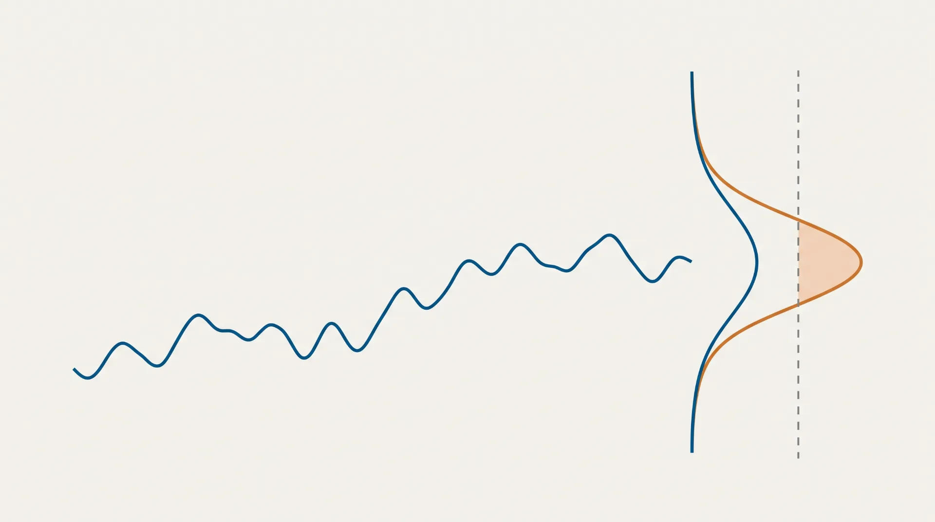
Two models, one number, opposite realities
Imagine you have a sensor recording something you care about, for example seismic background at a detector site, electrical load on a grid, or strain in a bridge cable, and you’ve trained a model to forecast the next value. The model looks at the recent history, thinks for a moment, and gives you a single number: .
There’s a threshold that fires an alarm. The question is: should you worry?
You can’t answer that. Not because you’re missing information about the model, but because the model is missing a way to tell you what it knows. That single number is all it can say. Let’s see why that’s a problem.
Imagine you actually have two models, both watching the same signal, both predicting at the same timestep. They even post the same mean squared error on your test set, not approximately, but identically to three decimal places. By every standard ranking metric, they are interchangeable. Except they’re not.
Here’s what’s hiding underneath.
-
Model A is looking at a moment where the true conditional distribution, the actual spread of values the signal could realistically take, given its recent history is very tight:
If this notation is new to you: is a Gaussian distribution (the classic bell curve), where is the center, and is the standard deviation, which controls the width. A small means the values cluster tightly around the center. Here, 99.7% of the probability mass sits within of the mean, roughly between 0.47 and 0.53. The threshold at 1.0 is 50 standard deviations away. That alarm will not fire in the lifetime of the experiment.
-
Model B is looking at a moment where the true distribution is wide:
Same center, but . The bell curve is now extremely spread out. The threshold at 1.0 is only standard deviations away. That’s nothing. Roughly 40% of the time, the signal will cross the alarm.
Same forecast. Same MSE. Same test set. But the actual risk of triggering the alarm is versus . If you’re deciding whether to evacuate, reroute power, or flag a detector event, those are opposite conclusions and the number you ranked both models with cannot tell you which is which.
The problem isn’t that either model is broken. Both predicted the correct mean. The problem is that a single number can’t express I’m sure versus I’m guessing and the reason the model can’t express that isn’t a training bug or a missing feature. It’s a direct, provable consequence of the loss function it was trained with.
That’s what this post unpacks. We’ll see exactly why MSE hands you the mean and discards everything else, what to replace it with, and what that replacement costs once a real optimizer gets hold of it.
···
What forecasting actually asks
Let’s set up the problem properly, because the assumption we’re going to break is hiding in the setup itself.
A time series is a sequence of numbers recorded in order over time.
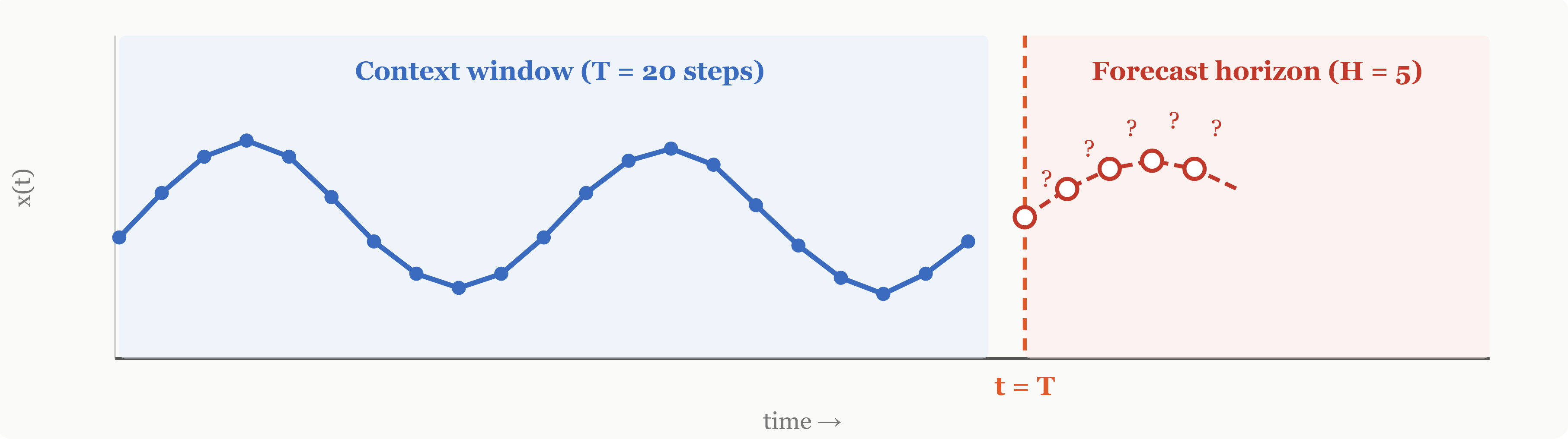
For instance, temperature every hour, stock price at market close each day, or displacement of a seismometer sampled at 100Hz. The key property is that the order carries information, the value at time tells you something about the value at . Shuffle the sequence and that information is destroyed. That’s what separates a time series from, say, a bag of independent measurements.
We write the observed sequence as:
where is the value at timestep . Forecasting means predicting the future values:
Two numbers control the setup:
-
= context length: how far back the model looks.
-
= forecast horizon: how far ahead the model predicts.
The simplest case is , which means predicting only the very next value. That’s where we’ll focus. In practice, can be dozens or hundreds, but the argument about MSE versus NLL applies identically regardless of .
Now here’s the subtle part that most textbooks gloss over. When you write down your prediction as a single number , you’ve made a philosophical commitment without realizing it. You’re treating the future as though it’s determined by the past, as though knowing the history perfectly would tell you the next value exactly.
Think about what that single number means. The model says the next value is 0.5, not probably around 0.5, not somewhere between 0.3 and 0.7, just 0.5, full stop. That format has no room for doubt. There is no field in the output for by the way, I’m not sure about this one.
Nobody agrees to this assumption on purpose. You agree to it by picking a loss function. The loss decides what the model can and cannot express, and the standard loss, MSE, decides for you: the answer is a point, not a distribution.
···
The simplest loss, and what it actually optimizes
The most natural thing a model can do is emit one real number for each future step. Training needs a loss function, that is, a way to measure how wrong the prediction was. The near-universal choice is of this problem is the mean squared error:
where the sum runs over all training examples and timesteps. It’s zero when the prediction is exact, and grows quadratically as the prediction drifts away:
-
An error of 2 costs four times an error of 1.
-
An error of 10 costs a hundred times an error of 1.
Large errors dominate the gradient, which is exactly what you want, miss the spike and you’ve missed the point.
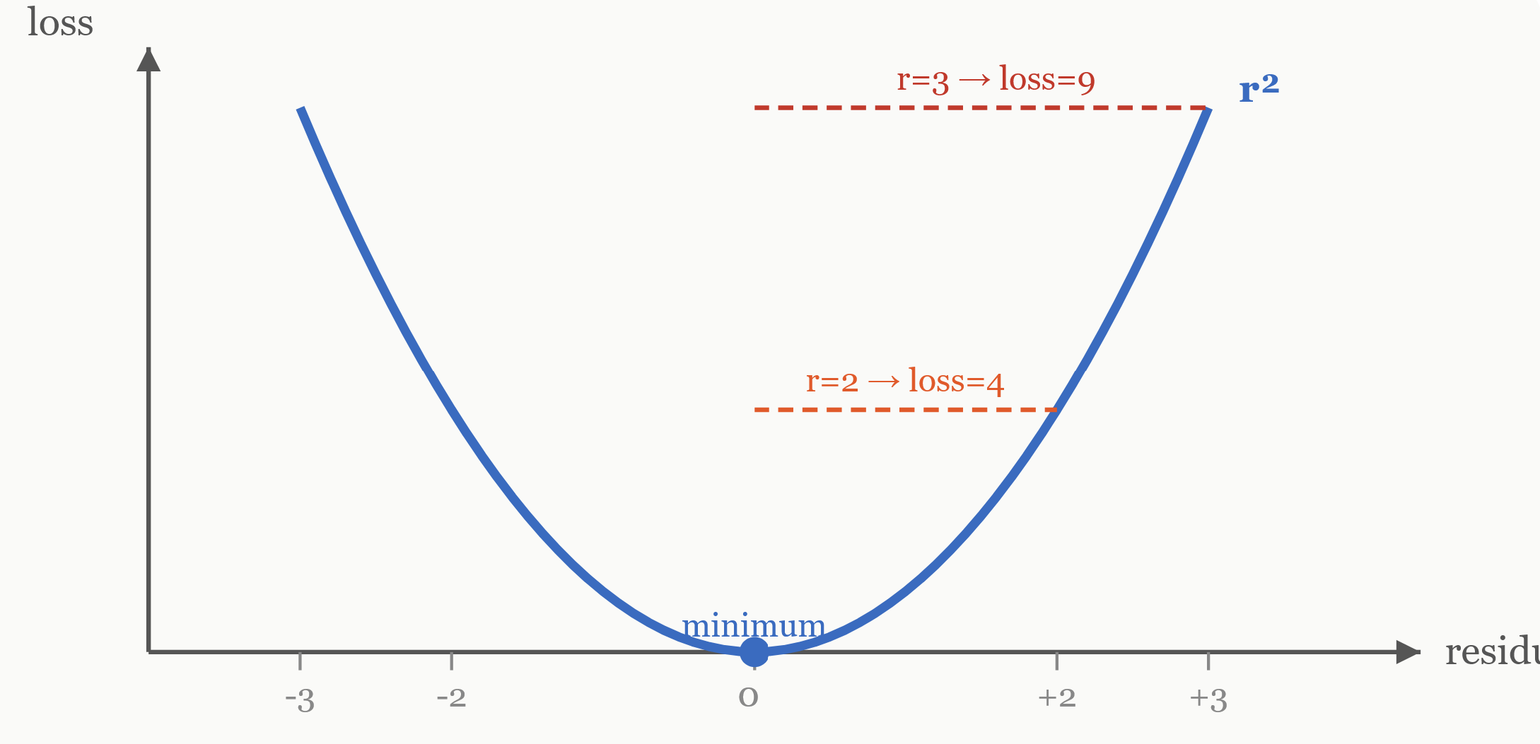
So far, so good. The trouble starts when you ask: what prediction does MSE actually reward? If the model could be perfect, what would MSE push it toward?
The proof: without history first
Let’s forget about neural networks, architectures, everything. Just pure math. Bear with me, the derivation is short, and it tells you something fundamental.
You have a random variable , the next value the signal will take. You don’t know what it will be, but it has some distribution with mean . Your model must commit to a single number. Think of it as writing one number on a piece of paper and handing it over, before the truth is revealed. Which minimizes the expected squared error?
We want to minimize:
Expand the square (just , then take the expectation of each term):
is a fixed number (depends on the distribution of , not our choice). is also fixed, that’s . So as a function of , this is a parabola opening upward. It has exactly one minimum.
Differentiate with respect to and set to zero:
The optimal single-number prediction under squared error is the mean. Geometrically: the point closest on average, in squared distance, to a cloud of possible outcomes is the center of that cloud.
Now with history
In forecasting, isn’t drawn from a fixed distribution. Its distribution depends on the history, that is, what the signal has been doing. Different pasts lead to different futures. Now, write for the observed history. Run the exact same argument, but condition everything on :
Differentiate with respect to , set to zero:
Nothing changed structurally. The derivation is exactly the same as before, we just added “” everywhere.
This is what the MSE optimizes for:
The MSE-optimal prediction is the conditional mean. This is what any model trained with MSE is pushed toward, regardless of architecture (transformer, LSTM, linear regression, anything). Given infinite data and enough capacity, the model converges to predicting the average of where the signal could go next, given the past it has seen.
The mean is a perfectly reasonable thing to predict. No other single number does better under squared error. But the mean is a single summary of location. It tells you where the center of the distribution sits. However, it tells you nothing about:
-
Width: Is the distribution tight ) or wide )?
-
Shape: Symmetric? Skewed? Heavy-tailed?
Two completely different situations can share an identical conditional mean and MSE, but by construction, cannot tell them apart. It has no term that rewards getting the width right, and no term that punishes getting it wrong. The spread is invisible to the loss. This is Model A and Model B restated in the language of the math. Same conditional mean, incompatible futures, one number.
···
The assumption nobody writes down
Here’s where it gets worse. MSE doesn’t merely ignore the spread, ignoring it would be survivable. Training with it is mathematically equivalent to assuming the spread is the same everywhere. To see this, we need a short detour through maximum likelihood estimation (MLE). Don’t let the name intimidate you, the idea is actually quite simple.
Maximum likelihood: the intuition
Forget loss functions for a moment and think about it differently. Your model, with parameters , looks at the history and makes a prediction. Instead of just asking how close was the prediction, ask a richer question: how probable did the model think the true outcome was?.
Say the true value turned out to be 3.7. A good model should have thought 3.7 was likely. A bad model thought 3.7 was a one-in-a-million event and then it happened, which means the model had a bad picture of reality.
Maximum likelihood just says: pick the model parameters that make the observed data as probable as possible. The settings under which reality looks least surprising. But to assign probabilities to outcomes, we need a noise model, an assumption about how observed values scatter around the prediction. The most natural starting point is a Gaussian with some fixed width.
The noise assumption
Assume that what you observe equals the model’s prediction plus random noise:
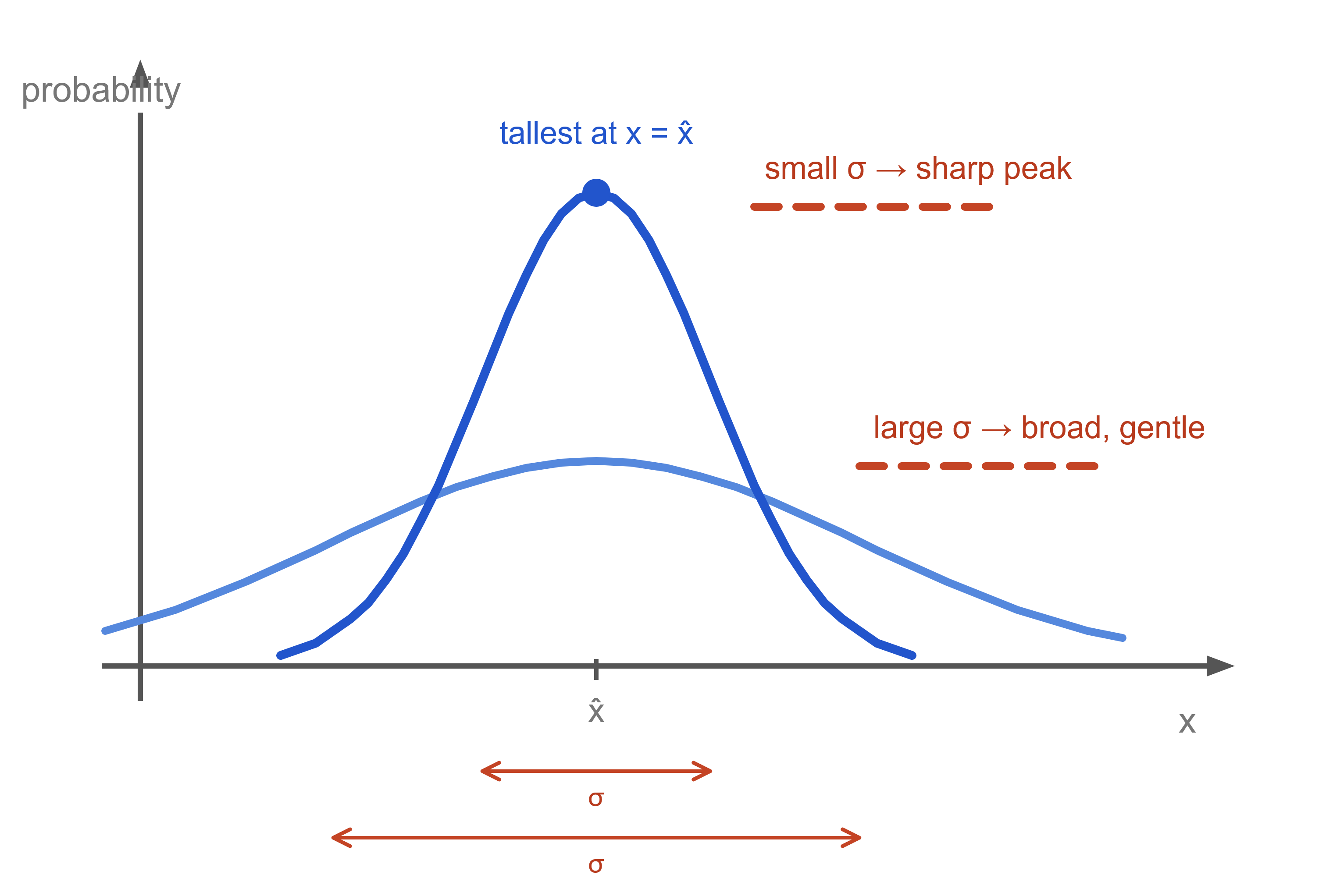
In words: the true value is the prediction, plus a small random perturbation drawn from a Gaussian centered at zero with variance . The key word here is fixed, the same for every data point, every timestep, every input. Under this assumption, the probability density of observing given the prediction is the Gaussian density:
If this formula is new to you: it’s tallest when (perfect prediction), and falls off as moves away from . The speed of falloff is controlled by , small means a sharp peak, large means a broad gentle curve.
From probability to loss function
Now you have independent observations. Each one has a probability under the model. The total probability of the entire dataset is the product:
Products of many small numbers underflow to zero on a computer, and their derivatives are messy. So we take the logarithm. Since is monotonically increasing, the parameters that maximize the product also maximize the logarithm. The product becomes a sum:
Plug in the Gaussian density. For a single term:
The first part is , which is the same for every data point (since is fixed). Sum over all observations:
Now, maximize over the predictions (i.e., over the model parameters). Look at the two terms:
-
First term: . Contains no at all. It’s a constant. Ignore it.
-
Second term: . The factor is a positive constant. It rescales but doesn’t change which parameters produce the maximum.
Strip both away, and maximizing the log-likelihood is precisely minimizing:
That’s MSE. Now read it backwards.
Every time you train with MSE, you have implicitly assumed that the residuals are Gaussian with constant variance , identical for every input. You made a probabilistic assumption. You never said it out loud. The loss function said it for you.
And once training ends, even that single is gone. It lived only inside the derivation. The trained model hands you and nothing else.
Why constant variance is almost always wrong
Think about what constant means in practice. The model is forced to be equally confident everywhere:
-
Forecasting electricity demand on an ordinary Tuesday night: easy, low variance. Forecasting it during a surprise heatwave: hard, high variance. Same for both? That’s the assumption.
-
Seismic background at a detector site on a quiet day: almost flat, very predictable. During a teleseismic event: wild fluctuations. Same for both? That’s the assumption.
The technical term for constant variance is homoscedastic. However, in a realistic situation, variance that changes with the input is heteroscedastic. Almost every real physical and economic signal is heteroscedastic. MSE can’t represent that.
This is exactly what separated Model A from Model B discussed above. The true conditional variance was in one case and in the other. An MSE-trained model fits one for the whole dataset and applies it everywhere, too wide when things are calm, too narrow when things are volatile, wrong in both directions. That’s the crack in the foundation, but, the fix is shorter than you’d think.
···
The leap: predict a distribution
The whole problem comes down to one thing: never appears in the model’s output. It was hiding inside the derivation that produced MSE, it was fixed to one value for the entire dataset, and it vanished after training. The model literally has no way to say I’m uncertain here.
The fix is very simple. Instead of emitting a single number, make the model emit the parameters of a probability distribution.
The simplest choice, and the natural one, given that MSE was already implicitly Gaussian, is two numbers:
where is the predicted center and the predicted width. The model now claims:
In words: I think the next value is drawn from a bell curve centered at with standard deviation.
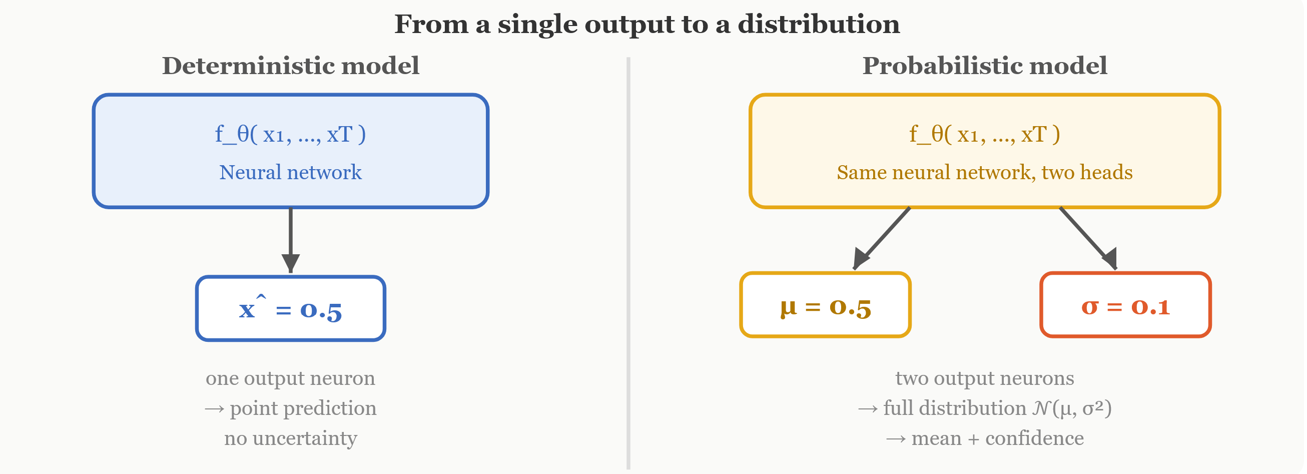
That is a bigger change than one extra output neuron suggests. The output space changes from (a single point on the number line) to a distribution over . The model stops committing to one answer and starts reporting a weighted range of possibilities, including how wide that range should be at this particular moment, given this particular history.
And is no longer a single global number. It’s a function of the input. The same model can output when the signal is in a calm stretch and when the signal enters a noisy regime. It gets to decide, at each timestep, how confident to be.
Architecturally, the change is minimal. The backbone, every attention head, every hidden layer, all the feature extraction, stays identical. The final layer gains one extra output neuron. One neuron produces , the other produces . That’s it. But now we need a new loss. MSE only knows how to compare one number to one number, it has no idea what to do with . If you train with MSE, the head will learn (MSE can score it), but the head will get no gradient signal at all. We need something that trains both.
···
Asking a better question
Your model predicts that the next value follows:
Then the true value is revealed. How do we score the prediction?
Forget formulas for a second. Think about it intuitively. The model drew a bell curve. That bell curve assigns a probability density to every possible outcome, high density near the center, low density out in the tails.
Then reality handed us a specific number . If landed near the peak, where the model put lots of probability, the model did well. It thought this outcome was likely, and it was right. If landed way out in the tails, where the model put almost no probability, the model did poorly. It was surprised by reality. So the natural score is: how much probability density did the model assign to the value that actually occurred?
That density is:
We want this to be large. Since is monotonically decreasing, maximizing this density is the same as minimizing the negative log-likelihood:
Why the logarithm? Two reasons. Practically: training minimizes losses, so we negate to flip maximize into minimize. In addition, numerically: likelihoods over many data points are products of small numbers (which underflow); turns products into sums, keeping things stable. Notice the shift in philosophy:
-
MSE asks: How far was your number from the truth?
-
NLL asks: How surprised should you have been by the truth, given the distribution you predicted?
The second question is richer because it involves both the center and the width.
Now let’s derive the formula. No tricks, just algebra. Bear with me, it’s just four lines and then we’re done. Start from the Gaussian density:
Step 1: take the logarithm: The expression is a product (fraction times exponential), so splits it into a sum:
Step 2: expand the first term. Using and:
Step3: assemble.
Step 4: negate and drop the constant. The term depends on neither nor , so its gradient is zero. Drop it:
Two terms, two jobs. And they don’t cooperate, they fight. The fight is the mechanism.
···
Two terms and the fight between them
Understanding this competition is the key to understanding every failure mode you’ll potentially meet later. Let’s take the two terms one at a time.
The fit term:
The numerator is the squared residual, exactly MSE. The new element is the denominator: , which is the model’s claimed variance (times 2).
Dividing by makes the penalty relative to the confidence the model claimed before seeing the answer.
Imagine the model predicted and the truth is . The squared residual is 1.0. Now:
-
(very confident): fit term . Enormous. The model said I’m certain, and was badly wrong.
-
(modest): fit term . The miss was within the claimed spread.
-
(very uncertain): fit term. Nearly free.
The model is allowed to make mistakes, but only if it admitted beforehand that those mistakes were possible. The value of was chosen before was revealed, no cheating after the fact. But here’s the catch. The fit term gets cheaper as grows. Always. For any fixed residual, a bigger means a smaller penalty. So if this were the only term, the model would discover a trivial strategy: set and never be punished for anything. This is obviously useless, a model that says I have no idea everywhere isn’t forecasting, it’s giving up.
The honesty term:
This closes that door. increases as increases. That’s it. That’s the whole mechanism.
-
Small (high confidence): is small or even negative. This reduces the total loss. The model is rewarded for precision.
-
Large (low confidence): is large and positive. This increases the total loss. The model pays a price for hedging.
The balance
Put both terms together:
The fit term says: make bigger so my errors cost less, while the honesty term says: make smaller so I get rewarded for precision. These two forces pull in opposite directions, and the model has to find where they balance. That balance is not a hand-tuned tradeoff. There is no hyperparameter weighting the two terms, they came from the same derivation, from the same logarithm of the same Gaussian density. The balance falls out of the math.
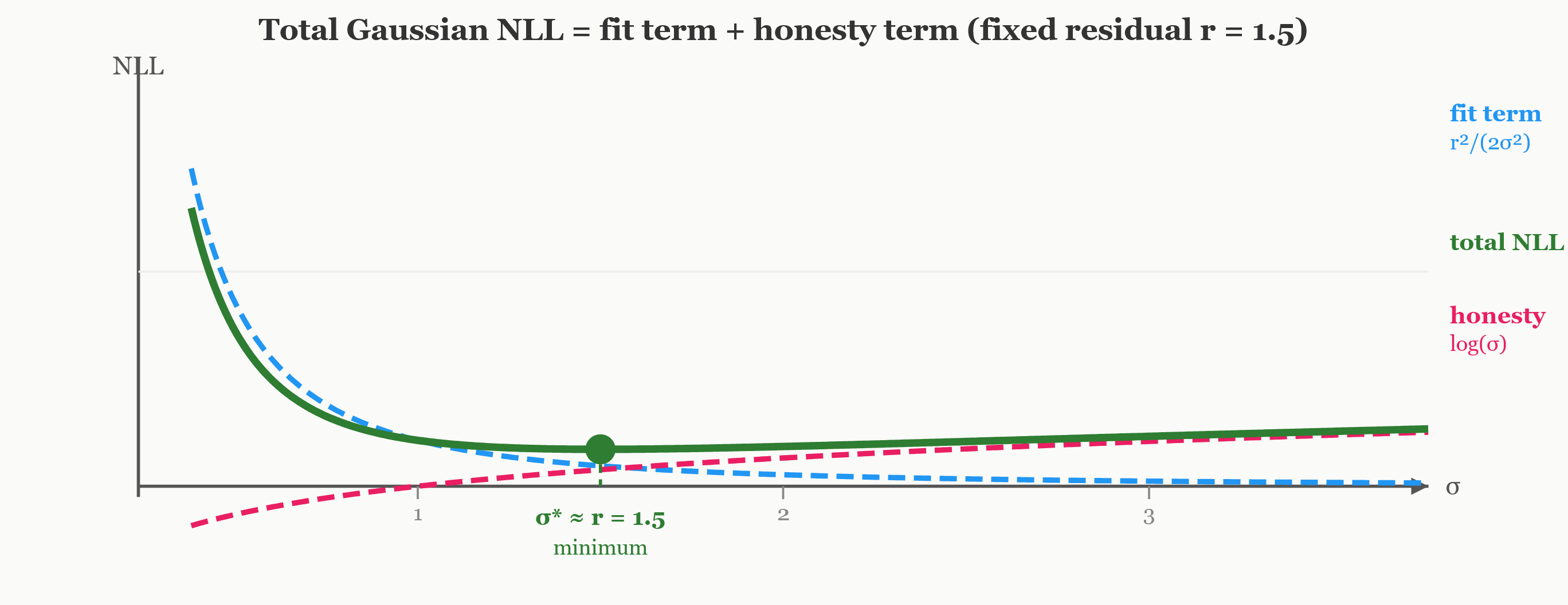
To make this concrete, fix the residual at and look at the total loss for different :
|
|
Fit term |
Honesty term |
Total |
|
|
|
|
1.557 |
|
|
|
|
1.125 |
|
|
|
|
0.905 |
|
|
|
|
0.974 |
|
|
|
|
1.224 |
|
|
|
|
1.654 |
The minimum is at , which is exactly , the size of the residual. At small , the fit term dominates. At large , the honesty term takes over. The sweet spot is where the model’s claimed uncertainty matches the actual error.
Wow, that’s not a coincidence. The next section proves it exactly.
···
What the optimum has to be
We’ve seen the intuition. Now let’s find the balance exactly.
Optimal
Hold fixed and optimize . The only -dependent part of the loss is:
This is MSE multiplied by the positive constant . Multiplying by a positive constant stretches the function vertically but doesn’t move the minimum. We already know MSE is minimized by the conditional mean, so:
NLL and MSE agree completely on where the center should be. The in the denominator rescales the penalty but doesn’t shift the optimum. Everything the model already knew how to do is preserved.
Optimal
Now fix and optimize . Define the true conditional variance:
This is how spread out actually is around its mean, given the input. It’s a property of the data, not the model. From ‘s perspective, is just a fixed positive number.
The expected loss as a function of :
Differentiate. The derivative of is .
The derivative of is :
Gaussian NLL pushes toward the true conditional variance.
The model learns both the conditional mean and the conditional variance simultaneously, one loss function, two targets.
This means the uncertainty is not a manually chosen constant. The model produces a different for every input, matching the actual local noise. When the signal is in a calm regime, is small and so is . When the signal enters a noisy regime, both grow. The model learns to be confident where it should be confident, and uncertain where it should be uncertain, automatically, from the data.
That’s the missing piece from Sections 1-4. Model A’s small variance ) and Model B’s large variance () can finally be distinguished, because the loss gives the model a reason to learn them.
···
Why this is the right loss, not merely a good one
Everything so far has been: here’s a loss, the math works out, the optimum is nice. But you could reasonably ask why this loss? Could you cook up a different two-term penalty that also balances and ? Something like with a hand-tuned ?
Indeed, that would also penalize large . It might even work okay. But it would be an arbitrary recipe with no principled interpretation. Gaussian NLL isn’t one recipe among many. It has a deeper justification from information theory.
KL divergence: the intuition
Let be the true conditional distribution (how reality actually generates outcomes) and the model’s prediction. The Kullback-Leibler divergence measures how different they are How much information is lost when you use the model’s distribution as a stand-in for the true one?
If they match perfectly, KL is exactly zero, no information lost. The more they differ, the larger the KL. The KL divergence is defined as:
Expand the log ratio:
The first term is the negative entropy of the true distribution, this is a fixed number that depends only on ground truth (reality), not on the model. From ‘s perspective, it’s a constant. The second term is the expected log-likelihood under the model. So:
The deep connection
When you minimize NLL, you are minimizing the information-theoretic distance between the model’s predicted distribution and the ground truth. You’re dragging toward .
In addition, KL divergence doesn’t just care about the mean or the variance. It cares about every aspect of the distribution, such as skewness, kurtosis, tail behavior, everything. The only reason we learn just mean and variance here is that we chose a Gaussian for , and a Gaussian is fully determined by those two numbers. Choose a richer family, and the same NLL principle pushes the model to learn those extra aspects too.
The cleanest way to see the fundamental difference:
-
MSE minimizes a distance between two numbers.
-
NLL minimizes a distance between two distributions.
MSE operates in the space of values. NLL operates in the space of probability distributions. The second is infinitely richer. And here’s the beautiful part: when you restrict NLL to a Gaussian with fixed , it collapses back to MSE, that was Section 4. MSE is a special case of NLL, the case where you’ve given up on learning uncertainty. NLL is the general framework; MSE is what you get when you freeze and throw it away.
···
Practical Engineering
Beautiful objective. Now make it survive when it works with an optimizer. To achieve this, two engineering details must be taken into account and one deeper issue stands between the derivation and the code that trains.
Predict , not
The output layer produces any real number, but must be strictly positive. How do you enforce that?
-
ReLU: . Positive (or zero), but terrible. For the output is zero, the gradient is zero, the network can’t learn. Half the range is dead. And is catastrophic, the fit term blows up to infinity.
-
Softplus: . Better, always positive, never zero. But the gradient saturates near , making learning sluggish exactly where precision matters.
-
The standard move: let the network predict (unconstrained, any real number) and recover . The exponential is always positive, smooth everywhere, and its own derivative. Rewritten in , the NLL becomes:
Both and now range freely over . Nothing for the optimizer to fight.
Clamp the range
Even reparameterized, can wander somewhere useless:
-
(): the fit term explodes on the tiniest residual. Gradients blow up.
-
(): the model claims total ignorance. Useless.
A simple clamp keeps things sane:
This gives , wide enough for normalized time series. The lower bound is called the -floor. If you see the model’s pinned at the floor across many inputs, something is likely wrong with the floor setting or the data normalization.
The optimization trap
This one is subtler. It’s not about numerical stability, it’s about the optimization landscape. Look at the gradient of the fit term with respect to :
See the ? The gradient that updates is scaled by the inverse of . When is well calibrated, this is fine. But early in training, here’s what happens:
-
The model starts with random parameters. Predictions are bad, large residuals everywhere.
-
Two paths to reduce the loss: improve (hard, requires learning signal structure) or increase (easy, just shift the output upward).
-
The model takes the easy path, grows.
-
As grows, the factor shrinks. The gradient on weakens.
-
The model stops improving for the hard examples, because it already labeled them as uncertain.
A vicious cycle: large weak -gradient stays bad large residuals justify large . The model learns to explain away its own mistakes by claiming uncertainty, instead of actually getting better. And the examples where this happens most are exactly the hardest ones, the ones the model most needs to learn from.
There are two practical fixes:
-
MSE warmup. Train with plain MSE first, ignoring the head. Once is reasonably accurate, switch to NLL. Now has a meaningful signal to learn from, and the shortcut of inflating is less tempting because the predictions aren’t that bad anymore.
-
-NLL. Multiply each sample’s loss by a detached factor of .
This reweights gradients so hard examples keep contributing even when is large. At you get standard NLL; at the weighting exactly cancels the effect. In practice is a good default.
The key lesson: a loss function can have a mathematically correct optimum and still be difficult to optimize in practice. Proving that tells you what the model should learn. It does not guarantee that gradient descent will get there.
···
Where the notebook picks up
Everything above is the derivation. Now the question we parked: does this actually happen when you train a real model?
The companion notebook builds two transformers with the same backbone, on the same synthetic signal. The signal is designed so that its noise level changes over time, quiet stretches and noisy stretches, and nobody tells either model where the boundaries are.
-
Model 1: trained with MSE. Outputs one number per timestep.
-
Model2: trained with Gaussian NLL. Outputs and .
On plain point accuracy, they finish nearly similar. We already predicted this: NLL and MSE agree on the optimal , so adding doesn’t hurt point predictions. On this metric alone, you’d call them interchangeable. But they’re not. Split the test set into quiet and noisy regimes. Ask each model to draw a 90% prediction interval, a band that should contain the true value 90% of the time. For the point model, the only option is one fixed band width computed from the global residual variance. For the probabilistic model, each timestep has its own , so the band is .
|
Quiet regime |
Noisy regime |
|
|---|---|---|
|
Point model (fixed band) |
|
|
|
Probabilistic model (learned ) |
|
|
The point model overshoots the 90% target when things are calm (the fixed band is too wide) and catastrophically undershoots when things are noisy (the band is far too narrow). One in three values that should be inside the interval falls outside. The probabilistic model stays roughly honest in both regimes, because its band actually tracks the local noise. Right on average, wrong where it matters. That’s the whole argument in one table.
The notebook also closes the circle on the threshold question from the opening. Given a threshold, the point predictor can only say yes or no. The probabilistic model returns a real probability, the quantity a decision actually needs. And there is a plot of the predicted widening and narrowing with the true noise. The model learned that from the data, because the loss gave it a reason to.
···
Conclusion
MSE is not a bad loss function. It does a good job of learning the center of the target distribution. But it says nothing about the uncertainty. never appears in the MSE formula. If the loss never sees uncertainty, it cannot learn it or evaluate it. That is, training with MSE implicitly assumes that the same amount of uncertainty applies everywhere, an assumption that is rarely true in real-world data.
Gaussian NLL fixes this by letting the model predict both and . The loss has two competing parts: one encourages the model to explain the data accurately, the other discourages it from claiming unnecessary uncertainty. Together, these forces drive the model toward the true conditional variance. Through the KL divergence connection, this objective isn’t a convenient heuristic, it minimizes the information-theoretic gap between the model’s distribution and reality’s. With one extra output neuron and a simple clamp, the model learns both the mean and the uncertainty in a single training run.
Two important lessons to carry forward:
-
First, predicted uncertainty is only as reliable as the optimization process that produced it. Even though Gaussian NLL has a correct optimum, training doesn’t always reach it. The weighting creates a shortcut that can trap early learning. Practical techniques, such as MSE warmup and -NLL, make the path to the optimum more reliable.
-
Second, the Gaussian is still an assumption. Predicting gives the model an input-dependent measure of uncertainty, but the predicted distribution remains unimodal (one peak) and symmetric (equal probability above and below the mean). Some problems don’t fit this shape. Imagine a ball balanced on a ridge: it could roll left or right, and the mean (the ridge top) is the one place it won’t stay. Data with multiple possible futures, sudden regime changes, or heavy tails requires richer predictive distributions than a single Gaussian can provide.
That is where more expressive approaches, such as quantized-token models and flow matching, become useful, and where the next part of this series begins. Until then, think back to the question we started with: Should I worry about this prediction? A model trained only with MSE has no meaningful way to answer. A probabilistic model trained with Gaussian NLL finally can.
···
References
[1] D. A. Nix and A. S. Weigend, Estimating the mean and variance of the target probability distribution, Proc. IEEE International Conference on Neural Networks, 1994.
[2] A. Kendall and Y. Gal, What Uncertainties Do We Need in Bayesian Deep Learning for Computer Vision?, Advances in Neural Information Processing Systems (NeurIPS), 2017.
[3] T. Gneiting and M. Katzfuss, Probabilistic Forecasting, Annual Review of Statistics and Its Application, 2014.
[4] M. Seitzer, A. Tesch, N. Rasiwasia, and G. Martius, On the Pitfalls of Heteroscedastic Uncertainty Estimation with Probabilistic Neural Networks, ICLR 2022.