

SIFT is one of the most widely known algorithms in computer vision. Its core objective consists of detecting object keypoints, generating descriptors for them, and matching the same objects across images.
As the name suggests, SIFT is a scale-invariant algorithm, meaning that the same object can appear at different scales in a pair of images, and SIFT will still be able to successfully detect its keypoints.
In addition, SIFT is rotation-invariant, making matching possible for rotated objects as well.
Let us take a closer look at how SIFT works under the hood.
Note: In this article, we will refer to the Laplacian of Gaussian (LoG) as a transformation used for edge detection in images. If you are unfamiliar with this technique, it is recommended that you go through one of the edge detection articles.
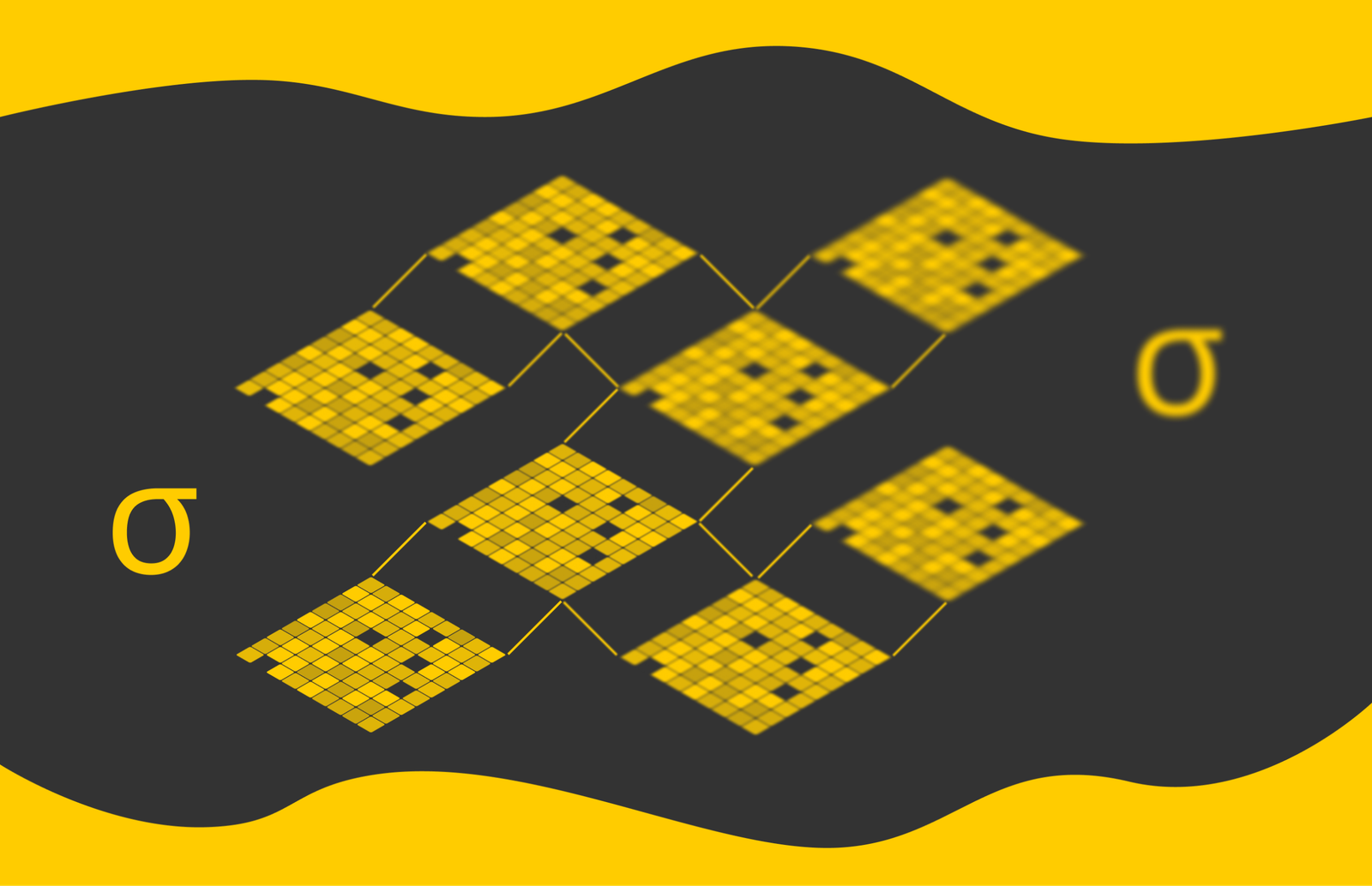
In its workflow, SIFT constructs several versions of the original image by applying resize and Gaussian blur transformations.
For simplicity, let’s imagine that I(x, y) is an original image. First, with chosen values of k and σ1, SIFT constructs several versions of the original image by applying Gaussian smoothing with different standard deviations: σ1, k⋅σ1, k2⋅σ1, k3⋅σ1, … , where k > 1.
This results in a sequence of images in which each subsequent image is slightly blurrier than the previous one. This sequence of images is called an octave.
Then SIFT computes the pairwise differences D1, D2, …, Dn between the resulting images, known as the difference of Gaussians (DoG). These differences highlight pixels with high intensity changes. After that, the algorithm stacks the Di and tries to find local extrema in them. Here is how it is done:
For each point in Di(x, y), SIFT examines its 26 neighbours:
-
8 adjacent points on Di level;
-
9 points directly above Di(x, y) (on the Di+1 level);
-
9 points directly below Di(x, y) (on the Di-1 level);
Then one of the following three cases is possible:
-
If Di(x, y) is greater than all of its 26 neighbouring points, then SIFT marks it as a maximum.
-
If Di(x, y) is less than all 26 neighboring points, then SIFT marks it as a minimum;
-
Otherwise, the point Di(x, y) is skipped.
For simplicity, the point Di(x, y) and its 26 neighboring points can be visualized as a 3x3x3 grid with the center at Di(x, y). This procedure allows the identification of the strongest features.
The found extrema values represent points of interest. In fact, there can be too many of them; that is why SIFT applies thresholding or another operator to retain only those that represent the greatest changes.
To account for different scale variations, the same process is repeated for an initial image reduced (downsampled) in width and height by a factor of two. As a result, a new octave sequence is constructed with greater Gaussian noise applied to it, having the following σ values: σ2, k⋅σ2, k2⋅σ1, k3⋅σ2, … , where σ2 = 2σ1. As before, extrema values are found from image differences using the 3x3x3 grid method.
For the third iteration, the image is downsampled again (reduced in width and height by a factor of two), and a new, blurrier octave is constructed with σ values as σ3, k⋅σ3, k2⋅σ3, k3⋅σ3, … , where σ3 = 2σ2 = 4σ1.
The entire process is repeated for a specified number of iterations.
We understood how to find points of interest. Let’s now answer several important questions to build intuition about the process.
Why DoG instead of LoG?
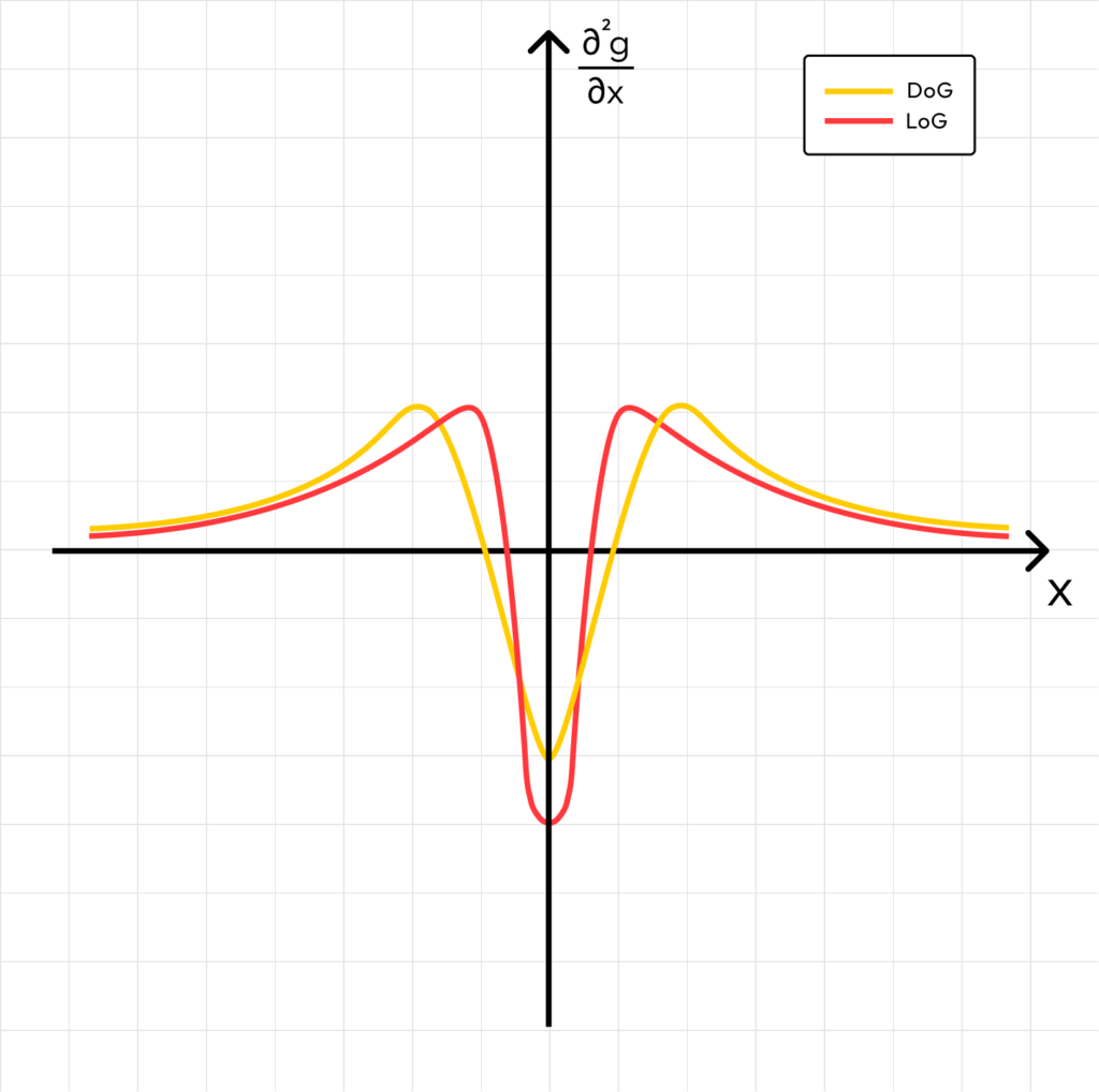
In the past, we found that the Laplacian of Gaussian (LoG) is a very useful transformation for identifying edges in images. At the same time, it turns out that there exists a very good approximation for the difference of two scaled LoGs applied to the same image:
DoG = nkσ – nσ ≈ (k – 1)σ2 ⋅ ▽2nσ
In fact, calculating DoG using this formula multiple times is much less computationally expensive than applying the original LoG formula each time.
Why construct several DoGs withing a single octave?
Within a single octave, image bluriness gradually increases. The difference between two consecutive DoGs highlights points of interest across scales.
For instance, a DoG constructed between a pair of consecutive net images (at the bottom of an octave) makes it much easier to detect smaller features. However, for larger features, this is difficult. For that reason, we also compute a DoG for more blurred images (at the top of an octave), where smaller features are not visible, and the algorithm focuses more on larger patches instead.
Why to construct several octaves?
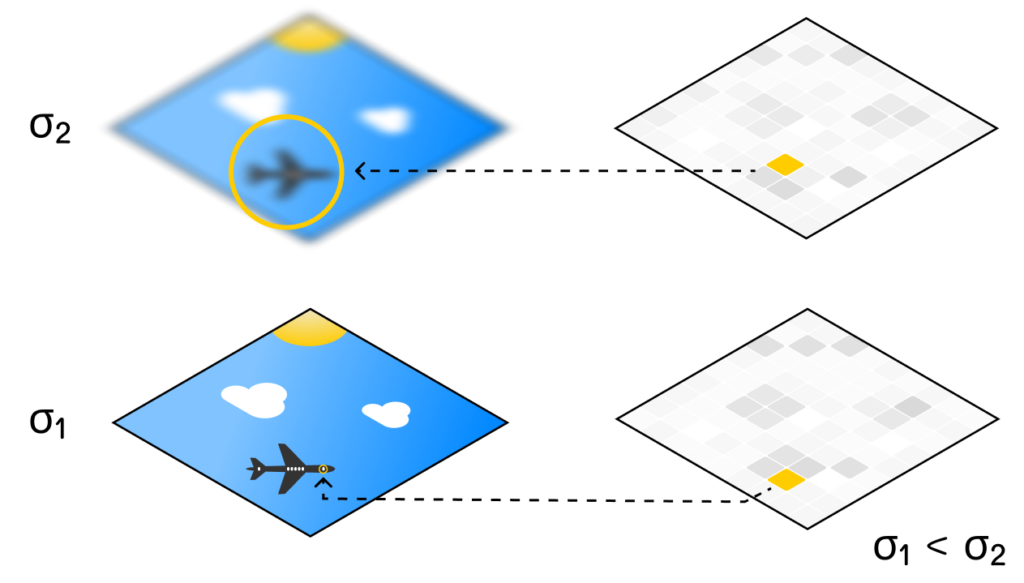
It is clear that as blur increases, we can detect larger features. So a natural question arises: why not just use a single octave, iterating from very small blur levels to very high ones? This way, we could detect features of all sizes.
The motivation for the construction of several octaves lies in two aspects:
-
As blur increases, small details become invisible in the image. So, in terms of efficiency, there is no point in keeping the full image resolution at higher levels of blur. Downsampling reduces the number of pixels by a factor of 4, making processing much faster.
-
Approximating very large Gaussian kernels can accumulate errors, so we shouldn’t use high values of σ. At the same time, downsampling can be roughly thought of as adding blur to the original image, since it also removes fine details. Given that, using higher levels of blur on the full-resolution image can be roughly equivalent to using smaller blur levels on smaller images.
Therefore, downsampling and octave construction provide significant advantages.
Why a 3-dimensional window?
A 3×3 window in a single image can detect local extrema, but there may be too many, especially since we also create multiple scaled versions of the image.
Adding a third dimension to the window ensures that the detected points of interest are distinctive not only on the 2D plane but also across different scales, making them stable under changes in image zoom.
If it’s unclear why finding extrema across DoG layers yields points of interest, a useful reminder is that DoG is an approximation of LoG, as defined above. At the same time, we explained in the edge detection article that image edges can be found at extrema after applying the LoG transformation.
After collecting all potential candidate points, SIFT filters out some of them. The problem is that even if a given point is an extremum, it can still be noise. To keep only the most meaningful ones, SIFT applies a threshold on intensity change to remove low-contrast weak candidates.
Once interest points are chosen, SIFT tries to construct descriptor representations for them that will allow these features to be matched across different images.
First of all, detected features across different DoG layers are mapped to circles of varying sizes, where the higher the σ value on the DoG layer, the larger the circle radius. Then, for all pixels in the original image within that circle, gradient directions are computed.
SIFT then divides the detected region into 4 equal quadrants and constructs a gradient direction distribution for each quadrant.
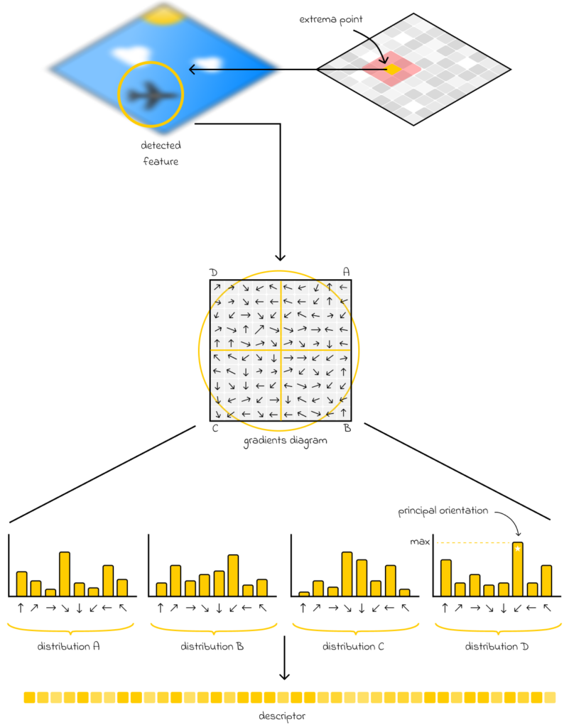
4 constructed distributions are then converted into a 128-dimensional vector, which is used as a feature descriptor for the initially detected feature.
For reference, SIFT provides robust internal mechanisms that allow it to handle situations in which a detected feature has fewer than 128 pixels. SIFT still enables computing a 128-dimensional vector descriptor by taking into account information from neighboring pixels as well.
A common case in real-world problems is when the same object appears in two images rotated by different amounts. To account for rotation correctly, SIFT also uses additional information about the principal orientation of the gradient, which is simply the most common gradient direction in the distribution. From a rotational perspective, this allows defining the starting point of the object, enabling correct mapping with others and helping avoid false-positive matches. These aspects guarantee the rotational invariance of the SIFT algorithm.
Comparing SIFT descriptors
SIFT descriptors are vectors that can be compared numerically to determine how similar they are to each other. The most common use case for descriptor comparison is determining whether the point of interest for which the descriptor is computed is the same across a pair of images.
L2-distance is a common choice for descriptor comparison:
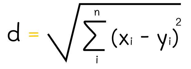
The lower the L2-distance, the better the match between two points. If the L2-distance is 0, the match is perfect.
Another useful metric is histogram intersection:
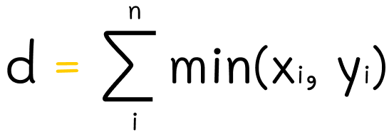
Here, the formula iterates through each vector component and finds the minimum of two values, which is equivalent to how well a particular aggregated gradient direction is present in both features. In this case, a higher metric value corresponds to better matching results.
Normally, the same objects across different images are expected to have many matches, making it possible to recognize their identity.
OpenCV provides an implementation of the SIFT algorithm. To create a SIFT object, the cv2.create_SIFT() method should be called. According to the SIFT documentation, several parameters can be specified:
-
nfeatures: the number of best features to retain. The features are ranked by their scores (measured in SIFT algorithm).
-
nOctaveLayers: the number of layers in each octave. 3 is the value used in the paper.
-
contrastThreshold: the contrast threshold used to filter out weak features in low-contrast regions. The larger the threshold, the less features are produced by the detector.
-
edgeThreshold: the threshold used to filter out edge-like features. The larger the edgeThreshold, the less features are filtered out (more features are retained).
-
sigma: the sigma of the Gaussian applied to the input image at the first octave.
Apart from the standard algorithm, we can easily visualize detected features on the image using the simple code snippet below.
Here is what the result looks like:

In reality, for more complex real-life images, the number of detected features can be much higher. Below is another example:
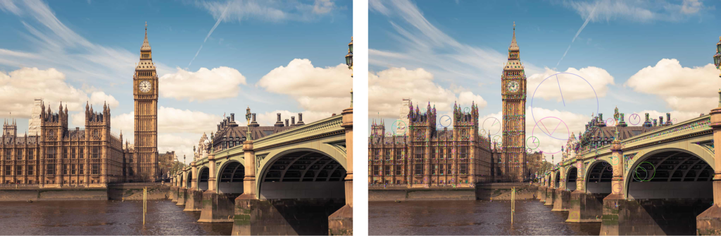
SIFT has a wide range of applications. Let’s look at them.
Image matching
As mentioned before, feature descriptors can be used for image matching. Let’s look at one example using the following image pair:

First, we will read a pair of images. Remember that before feeding them to SIFT, they must be converted to grayscale.
We then compute descriptors for each image.
Next, we’ll utilize BFMMatcher, or Brute-Force Matcher. This algorithm compares every descriptor in the first image with every descriptor in the second image, identifying the closest pairs based on the chosen distance measure. In our code, we’re using the L2-distance.
By calling the knnMatch() method, we pass all descriptors from both images and set k = 2, which specifies how many of the top k closest matches are returned for each descriptor.
The goal of setting the parameter k to a value greater than 1 is to remove less relevant matches by using Lowe’s ratio test.
The test consists of determining how good the best match is compared with the second-best match.
For instance, in the code below, we filter only good matches where the distance to the best match is less than the distance to the second-best match, scaled by RATIO = 0.75.
As it turns out, we can still end up with too many matches, so we keep only the best MAX_MATCHES = 50.
Finally, we can draw matches using the cv2.drawMatches() function.
Here is the result:

As we can see, SIFT did its job very well! It correctly matched the main objects in both scenes. A very interesting observation is that SIFT successfully preserved scale and rotation invariance!
For example, we can see that the plane was scaled and rotated differently in each scene. Despite this, SIFT produced very similar descriptors for each plane feature.
Object detection
Another SIFT application is object detection. With an object template, we can perform image matching in the same manner as above to search for that object in an image.
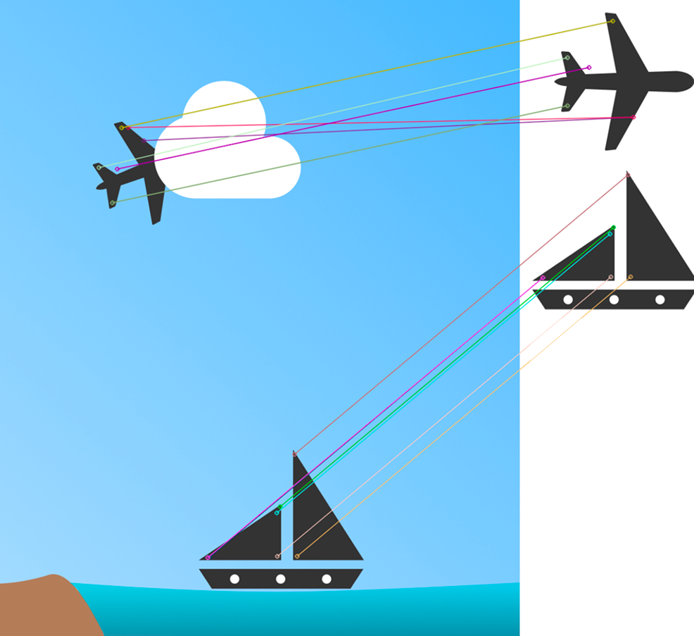
A great aspect of SIFT is that it tends to be robust against occlusions. If a part of an object is overlaid by another object, SIFT can still detect the visible features and match them successfully.
Once feature matching is complete, additional postprocessing techniques can be applied to extract the object’s contour and determine its precise location in the image.
It is worth noting that SIFT can sometimes produce false-positive matches, as shown in the image above. We can clearly see a red line connecting the airplane’s left wing in the scene on the left to its endpoint in the object template on the right, where it matches a point on the right wing.
Such situations can occur from time to time, and in most cases, they do not have a strongly negative impact. Depending on the task, postprocessing algorithms (e.g., RANSAC) can eliminate false-positive matches if there are not too many.
Image stitching
Image stitching is the task of merging photographic images taken from a single viewpoint that have overlapping regions into a single high-resolution image (a panorama). Image stitching can be elegantly solved with feature matching, perspective warping, and geometric transformations.
To do that, it is necessary to understand homography, which we will cover in one of the next articles.
3D-reconstruction?
While SIFT works very well for flat and 2D objects, it is unfortunately not suitable alone for matching 3D objects.
However, SIFT is used as one of the core steps in other 3D reconstruction algorithms (e.g., COLMAP). It allows matching points across images, from which the whole 3D scene is then constructed.
SIFT is a highly versatile algorithm for feature matching, notable for its capacity to match features while maintaining rotation and scale invariance.
As we saw, SIFT can solve a wide range of problems in computer vision. Image matching, object detection, and image stitching are among the most popular SIFT applications. In more sophisticated problems, SIFT is often used as a strong backbone for feature matching, which is then processed differently depending on the problem itself.
All images unless otherwise noted are by the author.