

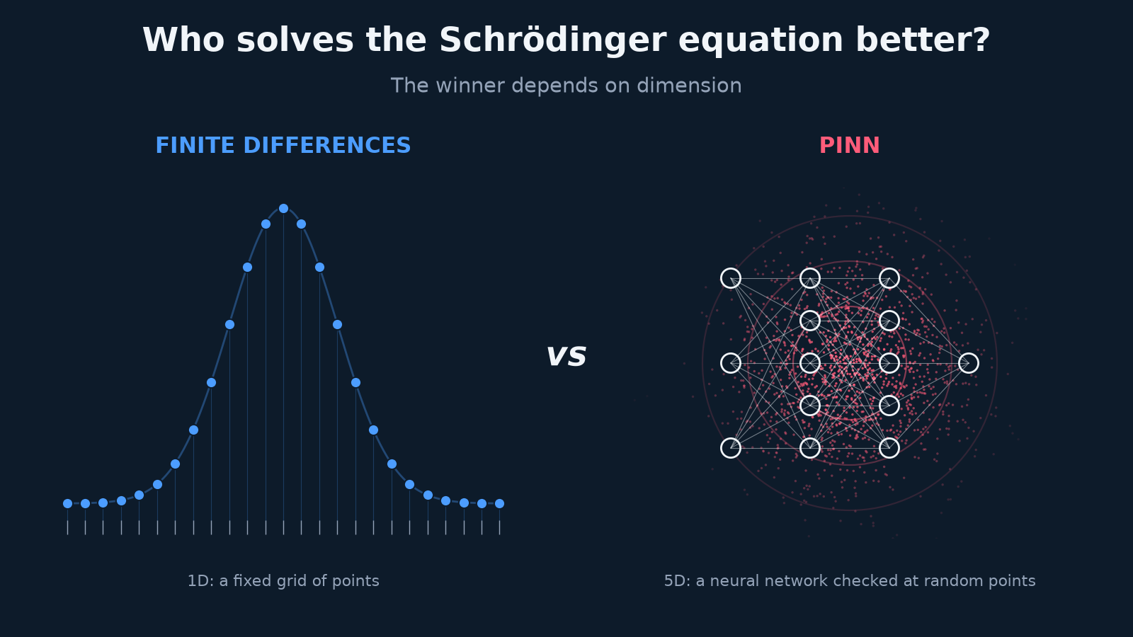
TL;DR
-
In 1D, finite differences win by about some thousands of times. They reach the PINN’s final accuracy in under a millisecond.
-
In 5D, the grid can’t compete. Matching the PINN’s 0.1% error would take about 5 billion grid points and more than 1 TB of memory. The PINN needed 89s of CPU time.
-
Two tricks made the PINN work. Switching from Adam only to Adam + L-BFGS cut its error by about 50×. So, forcing ψ > 0 stopped it from converging to an excited state.
Physics-informed neural networks, or PINNs, are everywhere right now. The concept is simple and easy to understand. You don’t need a mesh or a special solver. You write the equation into the loss function, and the network learns the answer.
I work in computational physics, and I kept asking one question: better than what? Many PINN demos never compare against a good classical method. A 2024 study in Nature Machine Intelligence found that weak baselines are common in this field, and that they make machine-learning solvers look better than they are. So I ran the test myself.
I picked a problem with an exact answer, the quantum harmonic oscillator. That way I can measure the error without any guessing. I solved it twice, first in one dimension and then in five. The two answers turned out to be very different.
The problem
Picture a marble rolling in a bowl. In everyday physics, the marble can have any energy at all. A quantum particle can’t. It can only sit on certain energy “rungs”, like steps on a ladder. Each rung has its own shape, called a wavefunction ψ(x). The square of ψ tells you where the particle is likely to be found.
The lowest rung is the ground state. It’s the one we want to find. The Schrödinger equation is the rule that decides which shapes and energies are allowed. For our bowl it is given as:
I use units where ħ = m = ω = 1. In d dimensions, the lowest-energy and its energy eigenstate is known exactly:
Don’t worry about the symbols, which perhaps look scary. Here’s all you need to know. H (in physics we call it Hamiltonian) is a recipe that takes a shape ψ and returns a new shape. The allowed states are the special shapes that come back unchanged, just multiplied by a number E. Mathematicians call this an eigenvalue problem. The solver must determine both the energy (E) and the corresponding wavefunction ψ. Therefore, one convenient approach is to place the particle inside a sufficiently large finite box and impose the boundary condition ψ = 0 at the walls. This artificial construction does not affect the physical result, provided that the box is chosen large enough. Although the wavefunction formally extends from −∞ to +∞, it decays exponentially at large distances. Therefore, for a sufficiently large box, the wavefunction becomes negligibly small near the boundaries, and the imposed boundary conditions have no significant effect on the calculated energy eigenvalues or wavefunctions.
The two contenders
Both methods both try to find the same curve. But they just look at it in very different ways.
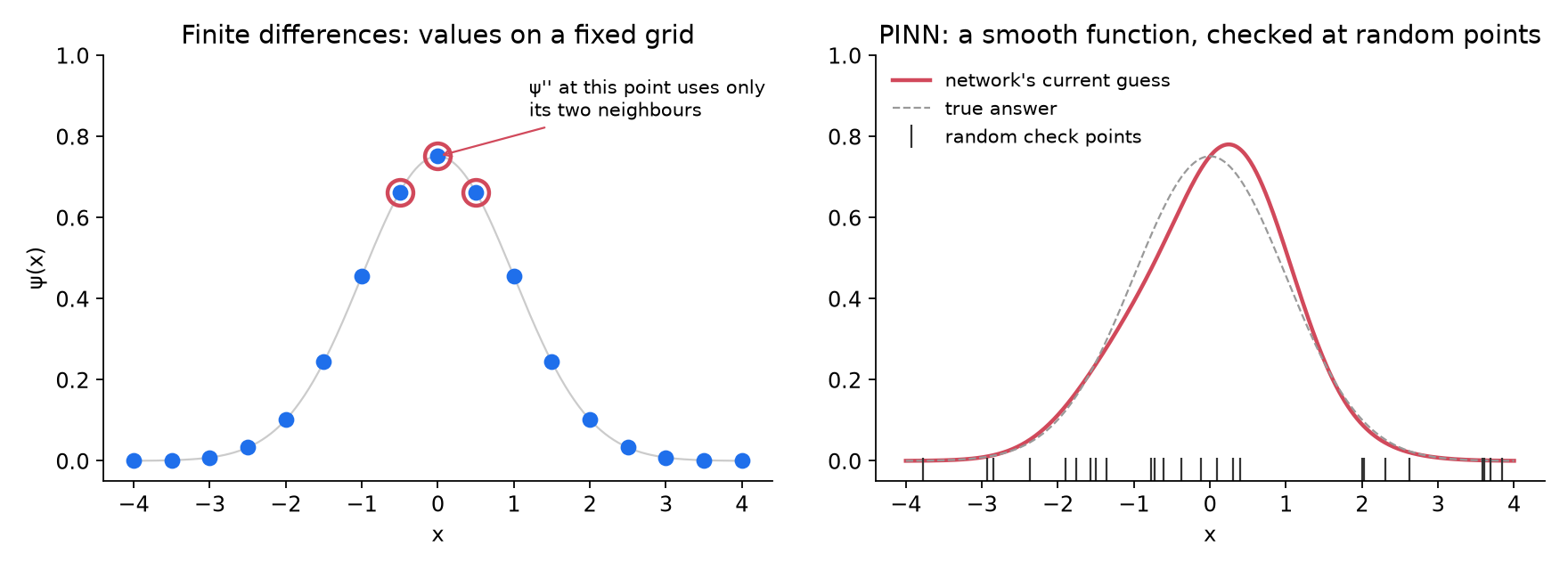
Finite differences method: I put N points along each axis and replace each second derivative with a simple formula that uses neighbouring points. The equation becomes a large sparse matrix, and we use SciPy to find its lowest eigenvalue.
There’s no training. The only choice is N. More points mean a better answer but a bigger matrix.
The PINN method: Here, a small neural network is the wavefunction. You give it a position x, and it returns a number ψ(x). At first its guess is random. Training improves it step by step, like this:
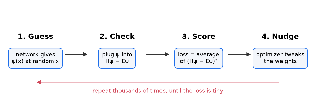
In practice, the loss asks it to satisfy Hψ = Eψ at random points. But, I compute E from the network itself with the Rayleigh quotient ⟨ψ|H|ψ⟩ / ⟨ψ|ψ⟩, so the energy always matches the current ψ.
Training has two stages. Adam runs first, on fresh random points at each step, to get roughly the right shape. Then L-BFGS, a quasi-Newton method, polishes the result on a fixed set of points. That second stage turns out to matter a lot.
I measured cost as CPU time on a laptop, not wall-clock time, so background load on the machine doesn’t distort the comparison.
In one dimension
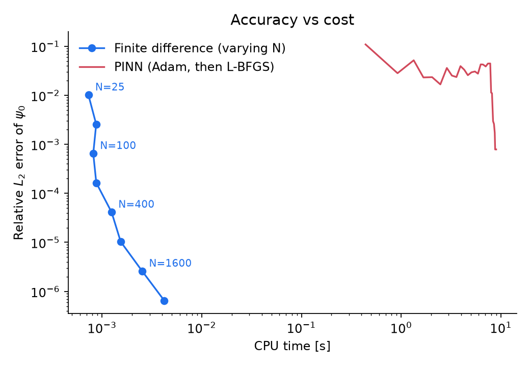
Both methods find the right ground state. The real question is how much each one costs.
In the below plot the axes are logarithmic, so each tick is ten times bigger than the one before. Points further left are faster, and points lower down are more accurate. The best spot is the bottom-left corner.
|
1D method |
CPU time |
Energy error |
Wavefunction error (L₂) |
|---|---|---|---|
|
Finite difference, N = 100 |
0.8 ms |
4.4 × 10⁻⁴ |
6.5 × 10⁻⁴ |
|
Finite difference, N = 1600 |
2.5 ms |
1.8 × 10⁻⁶ |
2.6 × 10⁻⁶ |
|
PINN, Adam only |
~8 s |
~10⁻² |
~4 × 10⁻² |
|
PINN, Adam + L-BFGS |
9 s |
5.7 × 10⁻⁶ |
7.9 × 10⁻⁴ |
Here two things are important and we must mention.
First, L-BFGS rescues the PINN. With Adam alone, the error stalls at a few percent. The loss just bounces around. When L-BFGS takes over, the error drops by a factor of about 50 within a few hundred iterations. If you want to take only one tip from this article, take this one.
Why does this happen? Think of training as walking downhill to the lowest point of a landscape. The PINN loss is built from second derivatives of the network, which autograd computes by differentiating twice. That makes the landscape stiff or ill-conditioned: it’s like a long, narrow canyon, very steep across and almost flat along its length. A first-order method like Adam only feels the local slope. So it bounces from wall to wall across the canyon and creeps slowly along it. That’s the noisy plateau in the training plot below.
L-BFGS is a quasi-Newton method. It also estimates the curvature, meaning how the slope itself changes, from its recent steps. With that information it can tell which way the canyon runs and take a long, confident step straight along it. For smooth physical problems like this one, that curvature information is close to essential. Adam is good for getting roughly into the right valley quickly but L-BFGS is what helps reache it to the bottom.
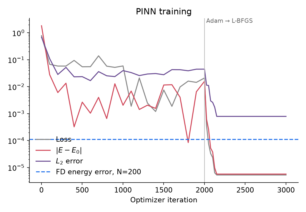
Second, finite differences still win easily. They match the PINN’s final accuracy in under a millisecond. That’s roughly ten thousand times faster. And turning N up keeps pushing the error down in a predictable way, while the PINN levels off.
The energy error is also much smaller than the wavefunction error. That’s expected as the Rayleigh quotient is variational, so a small error in ψ gives an even smaller error in E.
For this 1D problem, there is little practical reason to train a neural network.
In five dimensions
Now let’s make it harder. I took the same oscillator in five dimensions. The exact answer is still known: E₀ = 2.5.
“Five dimensions” sounds like science fiction, but it’s very ordinary in physics. Two particles moving in 3D space already need six numbers to describe them. Each extra particle adds three more.
Here’s the catch for the grid method. With N points per axis, a 5D grid has N⁵ points. With N = 16, that’s already a million unknowns. With N = 100, it’s ten billion. This is called as the curse of dimensionality.
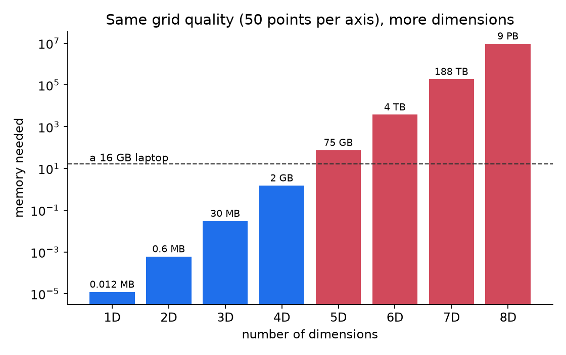
However PINN doesn’t need a grid. It samples random points, so its cost grows much more gently with dimension. In theory, this is where a PINN should shine.
Three things went wrong first
My first attempts at the 5D PINN failed. It needed some fixes, which are worth sharing, as they’re easy traps.
-
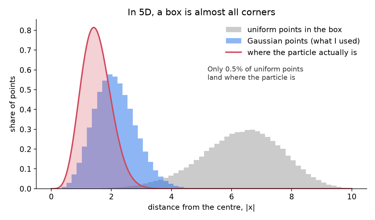
Uniform sampling wastes almost every point. In 5D, nearly all of a box’s volume lies far from the centre, where ψ is basically zero. So I sampled points from a Gaussian instead. The figure below shows why.
-
Importance weights blew up. To turn Gaussian samples back into box integrals, you normally weight each point by 1/p(x). In 5D, those weights ranged over about e⁴⁰. Out of 20,000 test points, only about 9 really counted. Therefore, I trained without the weights, which is still a valid way to enforce the equation. For testing, I drew points from |ψ₀|² itself, which keeps the weights well behaved.
-
The network found the wrong state. This one is surprising. The loss is zero for any eigenstate, not just the lowest one. My network happily settled on E ≈ 3.5, which is the first excited state. Although it was a perfect solution of the equation, but just not the one I wanted.
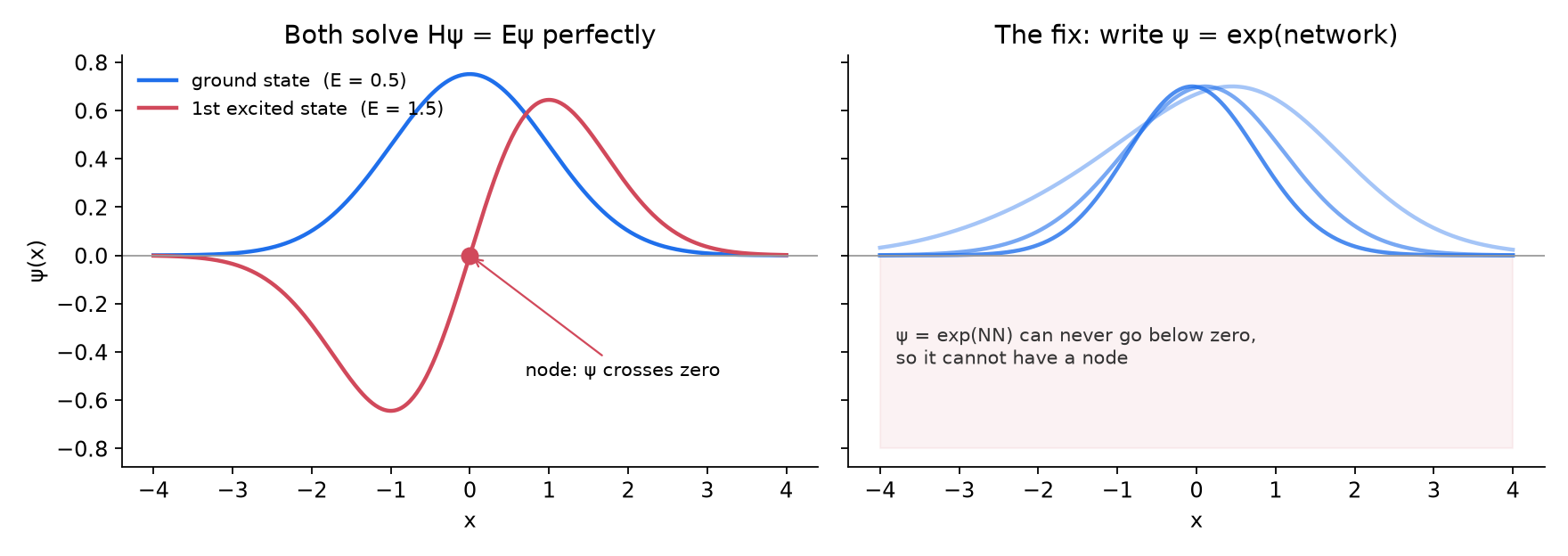
The last fix needs a small piece of physics. A ground state has no nodes, so it never changes sign. Therefore, I wrote the network as
The first factor makes ψ vanish on the walls. The exponential keeps ψ positive everywhere, so excited states are ruled out. I didn’t build in the Gaussian answer. The network still has to find the shape on its own.
The results
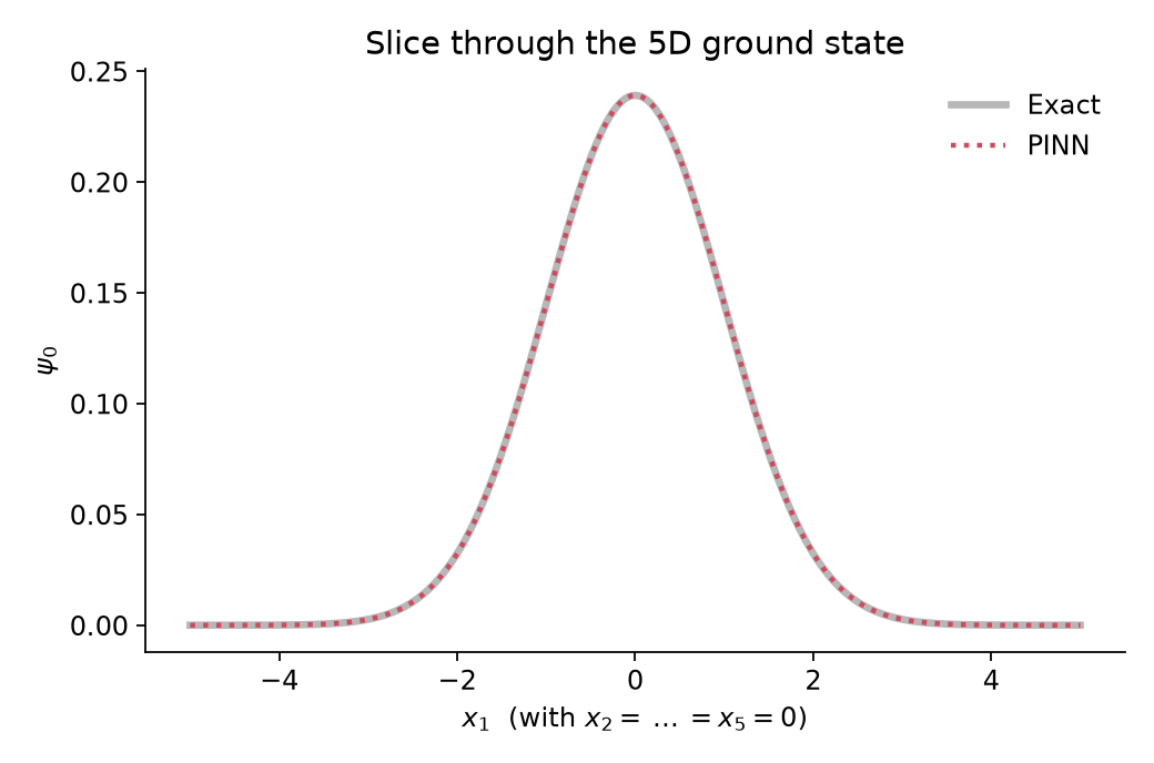
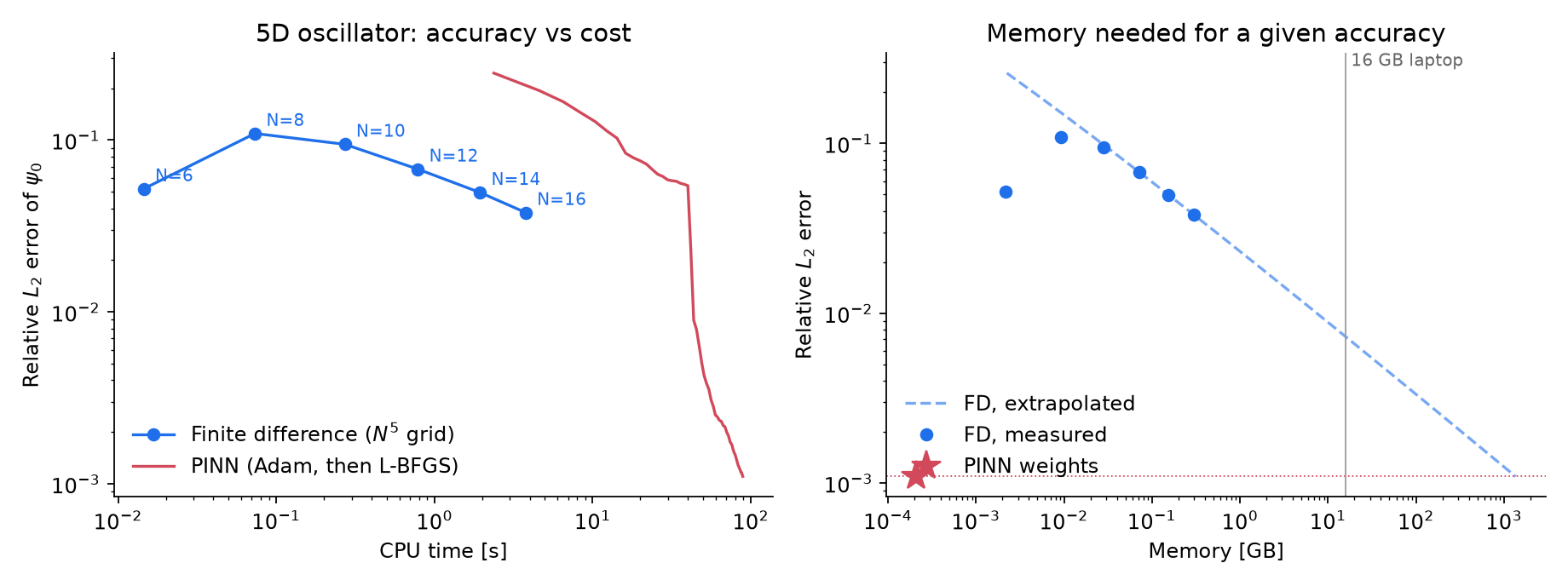
|
5D method |
Unknowns |
Memory |
CPU time |
Energy error |
L₂ error |
|---|---|---|---|---|---|
|
Finite difference, N = 16 |
1.0 million |
0.3 GB |
3.7 s |
5.5 × 10⁻² |
3.8 × 10⁻² |
|
Finite difference, N ≈ 86 (extrapolated) |
4.7 billion |
~1,400 GB |
— |
— |
~1.1 × 10⁻³ |
|
PINN, Adam + L-BFGS |
~9,000 weights |
< 0.1 GB |
89 s |
6.3 × 10⁻⁵ |
1.1 × 10⁻³ |
Now the picture flips.
The biggest grid I have solve (with N=16) in my laptop is with a million unknowns and reached about 4% error. The PINN reached about 0.1% in 89 seconds of CPU time. Its energy is right to five digits: 2.50006.
For finite difference method, the measured grid error falls like h², where h is the grid spacing. Extending that trend, the grid would need about 86 points per axis to match the PINN. That’s roughly 5 billion unknowns and more than a terabyte of memory. The PINN fits the whole solution into about 9,000 numbers.
In 1D the grid wins by a factor of ten thousand. In 5D the grid can’t even start.
Is this a fair fight?
Partly. Let me be clear about the limits.
The 5D oscillator is separable. It can split into five independent 1D problems. A smart classical solver that exploits this, using separation of variables, a spectral basis or tensor methods, would solve it almost exactly in milliseconds. So PINN beats a generic grid solver, not every classical method. I chose this problem because its exact answer lets us measure the error honestly, not because it’s hard.
The PINN’s real advantage shows up when the problem doesn’t separate, for example with interacting particles or coupled potentials. There, the smart classical tricks stop working, and you’re left with grids, basis sets or Monte Carlo. That’s why neural-network wavefunctions such as FermiNet and PauliNet have become a serious tool for many-electron systems.
Nevertheless, the PINN got some help. I used a physics prior (no nodes) and a careful sampling scheme. Without those, it failed. That’s typical. PINNs don’t work “out of the box” as often as the demos suggest.
The grid, on the other hand, got no help. I used plain second-order finite differences. A higher-order stencil would move the grid curve down, but it wouldn’t change the N⁵ scaling.
So which one is better?
It depends on the dimension.
-
In 1, 2 or 3 dimensions, use a classical solver. It’s faster, more accurate and completely predictable. You also get many excited states for free from the same matrix.
-
In higher dimensions, grids become impossible, and a PINN or another neural method becomes a real option. It still needs care: good sampling, a second-order optimizer and some physics built into the network.
-
Always check for structure first. If your problem separates or has symmetry, a classical method that uses it will beat PINN.
Therefore, my advice is simple. Whenever you see a PINN result, ask what the best classical baseline would have done with the same compute. If the paper doesn’t say, run the test yourself. In low dimensions it often takes ten lines of SciPy. One more point is worth noting — five dimensions are not special here. The same argument applies to any sufficiently high-dimensional problem. I use five dimensions simply as a convenient demonstration of how the computational cost of a tensor-product grid grows with dimensionality.
Finally, the reported CPU times should be interpreted as representative rather than absolute. Actual runtimes can vary depending on the hardware, software environment, processor load, and other processes running on the machine. The purpose of these timings is therefore to illustrate the relative computational cost of the two approaches, rather than to provide universally reproducible benchmark times.
Try it yourself
All the code is on GitHub: github.com/Samit1424/pinn-vs-fd-schrodinger. It has two short Python scripts:
-
schrodinger_pinn_vs_fd.py: the 1D comparison. It takes a few seconds of CPU time. -
schrodinger_5d.py: the 5D comparison. It may take a couple of minutes.
Together they reproduce every benchmark number and result plot above. Download them and run:
Want a real challenge? Add a coupling term such as 0.1·x₁²x₂² to the 5D potential so it no longer separates. (A linear coupling like x₁x₂ won’t do because a rotation of the axes separates it again.) Or try a double well, V(x) = (x² − 1)², in 1D. I’d like to hear how you get on.
References
-
M. Raissi, P. Perdikaris, G. E. Karniadakis, “Physics-informed neural networks: A deep learning framework for solving forward and inverse problems involving nonlinear partial differential equations,” J. Comput. Phys. 378, 686–707 (2019). doi.org/10.1016/j.jcp.2018.10.045
-
N. McGreivy, A. Hakim, “Weak baselines and reporting biases lead to overoptimism in machine learning for fluid-related partial differential equations,” Nat. Mach. Intell. 6, 1256–1269 (2024). doi.org/10.1038/s42256-024-00897-5
-
D. J. Griffiths, D. F. Schroeter, Introduction to Quantum Mechanics, 3rd ed., Cambridge University Press (2018), Ch. 2.3. doi.org/10.1017/9781316995433
-
R. J. LeVeque, Finite Difference Methods for Ordinary and Partial Differential Equations, SIAM (2007). doi.org/10.1137/1.9780898717839
-
R. B. Lehoucq, D. C. Sorensen, C. Yang, ARPACK Users’ Guide, SIAM (1998). (Used by
scipy.sparse.linalg.eigsh.) doi.org/10.1137/1.9780898719628 -
D. P. Kingma, J. Ba, “Adam: A method for stochastic optimization,” ICLR (2015). arxiv.org/abs/1412.6980
-
D. C. Liu, J. Nocedal, “On the limited memory BFGS method for large scale optimization,” Math. Program. 45, 503–528 (1989). doi.org/10.1007/BF01589116
-
P. Rathore, W. Lei, Z. Frangella, L. Lu, M. Udell, “Challenges in training PINNs: A loss landscape perspective,” ICML (2024). arxiv.org/abs/2402.01868
-
S. Wang, Y. Teng, P. Perdikaris, “Understanding and mitigating gradient flow pathologies in physics-informed neural networks,” SIAM J. Sci. Comput. 43, A3055–A3081 (2021). doi.org/10.1137/20M1318043
-
R. Bellman, Dynamic Programming, Princeton University Press (1957).
-
A. S. Krishnapriyan, A. Gholami, S. Zhe, R. M. Kirby, M. W. Mahoney, “Characterizing possible failure modes in physics-informed neural networks,” NeurIPS (2021). arxiv.org/abs/2109.01050
-
D. Pfau, J. S. Spencer, A. G. D. G. Matthews, W. M. C. Foulkes, “Ab initio solution of the many-electron Schrödinger equation with deep neural networks,” Phys. Rev. Research 2, 033429 (2020). doi.org/10.1103/PhysRevResearch.2.033429
-
J. Hermann, Z. Schätzle, F. Noé, “Deep-neural-network solution of the electronic Schrödinger equation,” Nat. Chem. 12, 891–897 (2020). doi.org/10.1038/s41557-020-0544-y