Introduction to Reinforcement Learning: Multi-Armed Bandit Simulation in Python

Having machines learning by themselves is the ultimate Science Fiction dream. Today that gap is closing, with programs like AlphaGo and the different LLMs that are out there, but would you believe it if I told you researchers started formulating these kinds of problems and developing algorithms to tackle this in the late 1950s?

While that timeframe seems way too early in the history of technology and, at the same time, not that long ago, that’s actually when researchers started to formulate what would become Reinforcement Learning as we know it.

Reinforcement Learning (RL) is a type of Machine Learning where an agent learns optimal behavior through interaction with its environment. Rather than relying on explicit programming or labeled datasets, this agent learns by trial and error, receiving feedback in the form of rewards or penalties for its actions. This process mirrors how people typically learn naturally, making RL a powerful approach for creating intelligent systems capable of solving complex problems. [1]

This is a very interesting and complex topic, involving agents that learn to navigate their environment, while trying to maximize their rewards. So I thought the definition above, from the Google Cloud documentation, was perfect to succinctly summarize Reinforcement Learning’s purpose, challenges and goals.

Let’s start unpacking it.

How did we get to Reinforcement Learning

If we look back, what we know today as Reinforcement Learning, actually has its origins in the area of optimal control going back to the 1950s[2]. However, there were a couple of other areas of research that eventually led to the development of Reinforcement Learning [2]. Different areas of research interested in formulating methodologies and developing algorithms that would learn over time.

While the area of optimal control may sound unfamiliar to many (me included), you might be more familiar with one family of algorithms that was developed to solve these types of problems, Dynamic Programming.

Richard Bellman was researching methods to solve optimal control problems which, in essence, aim to design a controller following a specific set of rules, that minimizes a measure of a dynamic system over time. From his seminal work Dynamic Programming became an emergent area of study and many algorithms were developed, such as the Bellman-Ford and Floyd-Warshall algorithms.

The intersection of optimal control, dynamic programming and learning only emerged later, in the late 1970s. Paul Werbos developed Heuristic Dynamic Programming and then, a decade later, Chris Watkins integrated dynamic programming methods and online learning [2].

The field continued to evolve with key contributions from Dimitri Bertsekas and John Tsitsiklis, who coined the term neuro-dynamic programming in the mid 1990s. 

This continues to be an extremely active area of investigation, with applications ranging from robotics[3], programs like AlphaGo (experts at playing the game of Go) and Natural Language problems[4], just to name a few.

Key Features and Challenges

Not all Machine Learning problems are created equal, and there are three major characteristics that distinguish Reinforcement Learning problems from other Machine Learning problems. 

The first characteristic is that Reinforcement Learning problems are closed-loop problems, since everything happens within the system that includes the agent and the environment. The agent takes actions over the environment and those actions both inform and affect future states of the environment and its inputs. 

Another characteristic is that the agent is not given a clear set of instructions. It gradually discovers which actions to take, such that its goal, i.e., maximizing the reward, can be achieved. 

Lastly, the consequence of the agent’s actions on the environment may not be immediately seen [2]. Like when you’re in an IKEA store and you take a left, because that seems like the best action to take given your limited knowledge of the floor plan, only to discover that you reached a dead-end and have to be that person who awkwardly walks against the natural traffic of the store. Guilty as charged 😊

Exploration vs Exploitation

The agent doesn’t know from the get-go which rewards they’ll get at every point in time, they only learn about it as they explore the environment, and the trade-off between exploration and exploitation is something that sets Reinforcement Learning apart from other Machine Learning algorithms.

To obtain a lot of reward, a Reinforcement Learning agent must prefer actions that it has tried in the past and found to be effective in producing reward. But to discover such actions, it has to try actions that it has not selected before.[2]

So the agent needs to learn how to exploit the actions that give it the highest reward, but they only get to identify those high-value actions when it explores the environment.

At the same time, the agent learns how to balance getting the maximum reward in the long-term, rather than always taking the action that maximizes their reward at each specific point in time.

This is the underlying premise for agents in Reinforcement Learning algorithms.

Formulating Reinforcement Learning Algorithms

So far, you know Reinforcement Learning is all about an agent taking actions in an environment, but that’s still not enough to formulate a Reinforcement Learning Algorithm.

The agent is this entity that is moving through an environment and, at every point in time, observing what’s around them, the possible actions it can take and, after taking action, either getting a reward or penalty.

Thinking about it as a system, besides the agent and the environment, there are a few other components at play:

• State

• Policy

• Reward Signal

• Value Function

• Model of the environment

All of these components are important, but I’d say the State underlies all of them. In this case, State refers to how the environment, the agent’s world, looks to the agent at any point in time. 

Every time the agent takes an action in the environment, it is affected, it changes. The agent changes the State of the environment and, therefore, they are only able to take the actions that are possible or available to them in that state. The reward or penalty they’ll get is also specific to that state.

In order to take action, the agent must have a Policy. This is like a rule book the agent has to follow in order to pick one of the actions possible or available to it in each state. For example, in an environment made of a 4×4 grid you can represent a labyrinth the agent needs to traverse to get from Start to Finish. As the agent moves around in the environment, its Policy also gets updated with the knowledge it has been gathering along the way.

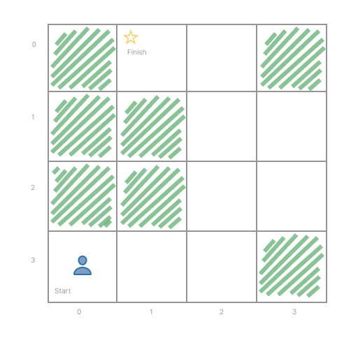
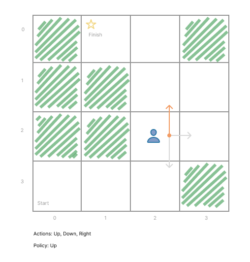
Each step of the way, the agent executes the policy and receives either a reward or a penalty. The policy could be a probability of taking a specific action on a given state of the environment, e.g., the agent has an 80% probability of going Up if they are on cell (2,2) compared to 20% for going Right when they are in (2,2). In case of deterministic policies, it maps to the specific action the agent should take. For instance, when the agent is on cell (1, 2) should go Up.

But what actually determines if the action the agent took is a reward or a penalty?

That is the Reward Signal [2]. As you can intuit by now, it’s something intrinsically dependent on the state of the environment and the specific action taken by the agent. Meaning, the same action taken in different states of the environment can have different reward signals.

While the Reward Signal provides immediate information to the agent, e.g. the action resulted in a reward or penalty, the Value Function determines how the agent is doing towards their goal in the long run. The value of the specific state the agent is in is, therefore, determined by the amount of reward the agent is going to accumulate over time, starting on that specific state.

At the end of the day, that’s what’s important. The agent’s goal is not to maximize the reward locally, i.e., at every single step but, to maximize it in the long run. 

Take our labyrinth for example.

In the first grid, at the starting point, when the agent is in cell/state (0,0), an action Right takes it to (0,1), which is in the path towards the end of the labyrinth, so it will have a higher value. However, looking at the second grid, when the agent is in (2,2) the action Right actually puts them in a dead end it will probably have to backtrack from. The action Right it has a negative or a lower value compared to the action Up when the agent is in (2,2).

Tying it back to Reinforcement Learning’s major characteristics, an agent that is purely greedy may be focused on the action that gives it the highest possible value that they know of, at every single step or state in the environment. By sticking with this action, in the long run, the agent might be actually be getting lower value rewards from each state, which contrasts with what it believes is the best action.

Back to IKEA, taking that left turn in a busy part of the showroom seemed like the best option, but it led you to a dead end! There was an immediate reward, i.e., getting away from the crowd, but that action resulted in a lower value in the long-run because you ended up backtracking.

Lastly, some Reinforcement Learning algorithms, called Model-based algorithms, will have a model of the environment. At each step, based on the environment state and an action, the model is able to predict the next state and the next reward. This model is used in planning, such that the agent can decide what action to take by predicting each possible state without actually having to explore it [2].

In this article we’ll be focusing only on Model-Free or Trial-and-Error Reinforcement Learning, where there’s not a model of the environment to guide the agent’s decisions.

To see how Reinforcement Learning algorithms show up in the real world, let’s take the Multi-Armed bandit problem with pertinent applications ranging from displaying ads or banners in websites, A/B Testing, to Dynamic Pricing [6].

Multi-Armed Bandit

This type of problem, also referred to as n-Armed Bandit, is a great example of the trade-off between exploration and exploitation.

It gets its name from being an analogy to a slot machine with many arms, instead of just one. Every time there are n choices, and it’s like pulling one of many levers in the slot machine. 

After each choice is picked, i.e., the action is taken, a reward is granted from a stationary probability distribution [2]. And, as you are probably expecting by now, each action has an expected value and the objective is to maximize the reward over a period of time.

The agent typically doesn’t know the true value for each action, otherwise it would have more chances beat the slot machine at its own game. Each arm pull has a random chance of being a win, but the agent would be locked in on the actual best arm. Instead, it creates an estimated value for each action based on its previous actions. And this makes sense, the agent only knows what it has observed so far in the environment as a result of its actions.

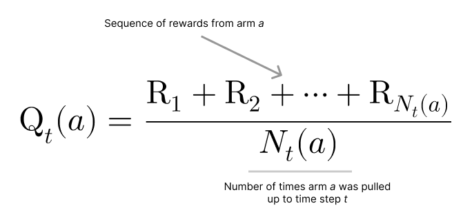
The estimated value at each step is the average of all the rewards received (cumulative) from the arm that was pulled in that particular step.

In practice, the agent can have two major tactics to play the multi-arm bandit, this multi-arm slot-machine. It can either be greedy or near-greedy, i.e., exploring different paths as it goes along.

In case the agent adopts the greedy approach, it always picks the arm with the highest estimated value it knows of, e.g., I picked the arm number one and it was a win, so that’s the highest value I know of and I’m sticking with it. This way it is exploiting an action it thinks is the best, given its previous knowledge which was pulling the arm number one exactly once. For all the agent knows, that looks like the best option.

If the agent has a near-greedy approach, from time to time, it will explore pulling other arms to see what is out there, with a certain probability, called epsilon. That’s why the near-greedy agent is also referred to as epsilon-greedy agent.

The trade-off between exploration and exploitation comes from the fact that the agent is basing its actions on previous knowledge. It ultimately depends on the agent’s approach, if it wants to exploit the information it already knows, or if it wants to explore, gaining more information about the effect or outcome of different actions. 

The greedy approach takes the result of the first pull that resulted in a win at face value. Meaning, whichever was the first arm it pulled that resulted in a win, it takes as the best action, the action that results in the highest reward. It observes that single piece of information and runs with it. Whereas in the near-greedy approach it gathers information as it goes. It may get a lower reward for a bit, but the information it gains about the different actions could result in a higher reward in the end.

Exploring different actions may be a great strategy in the long run. However, if the greedy agent lucks out and, in its first pull that is a win picks the arm that is actually the best, on average, the near-greedy agent won’t be able to beat the outcome of the greedy agent. Since the near-greedy agent will always spend a portion of the time exploring different arms, while the greedy agent is locked-in on the best arm, i.e., the arm with the highest true win rate.

To understand the mechanics of the estimated expected value, let’s take and agent that pulls a lever 5 times, in a 2-arm bandit.

But first a bit of nomenclature. The true value of an action a, what the agent never knows in advance, is typically referred to as q(a), and the estimated value the agent calculates at each step, to make decisions off of, is referred to as Q_t(a) meaning, Q(a) at the time step t. At every point in time t, the agent calculates it as:

In the image below, you can see the actual values for each arm pull. As mentioned before, the agent won’t know about the value of their action until they execute it. Showing the values for each possible action here is merely an illustration of the exploration vs exploitation trade-off.

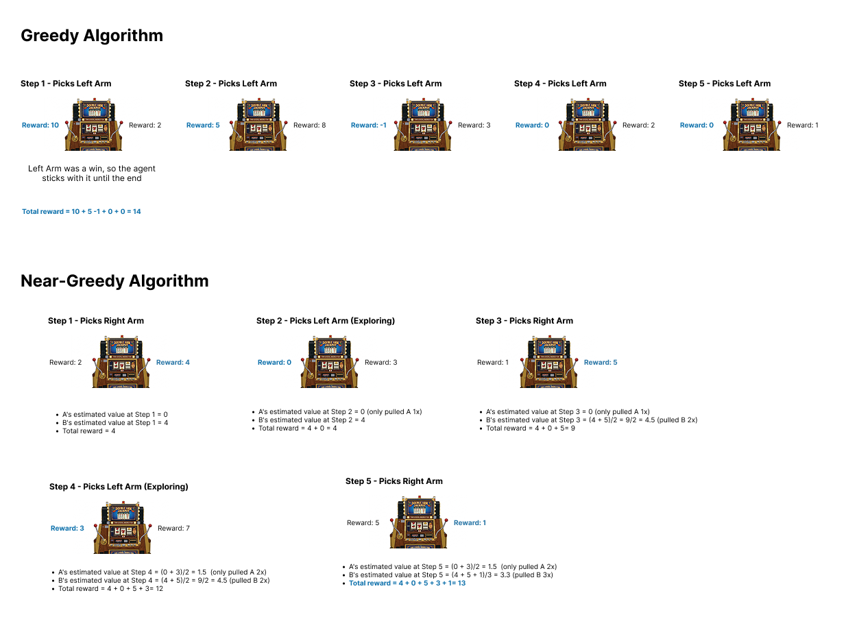
In the image above you can see the greedy agent was lucky on its first pull, that it had a win. Then it stuck with that arm and beat the near-greedy agent, which was not as lucky in its exploration. In the end the greedy agent had a total reward of 14, compared to 13 for the near-greedy agent.

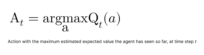
In a greedy approach, the agent will select the action with the highest estimated value. So, at time step t, it will select the greedy actions At, such that:

This is great so far, but you might be wondering Who sets these rewards?

The answer is, there’s not a single approach.

In practice, there are several ways to model the Reward system [6]. For instance, Independent and Identically Distributed (IID) rewards are each drawn independently from a fixed distribution. Here, the reward only depends on the arm that is pulled. 

But you can also set arbitrary rewards, i.e. Adversarial Rewards, which mimics the rewards an adversary would pick as they were trying to trick the algorithm.

Or you can model it as a Random Process, in which the state of each arm evolves over time as a random process, like as a Random Walk or a Markov Chain.

The Multi-arm Bandit Simulator

To explore a bit more the details of the see Multi-arm Bandit problem and observe the trade-off between exploration and exploitation, I created a Multi-Arm Bandit simulator.

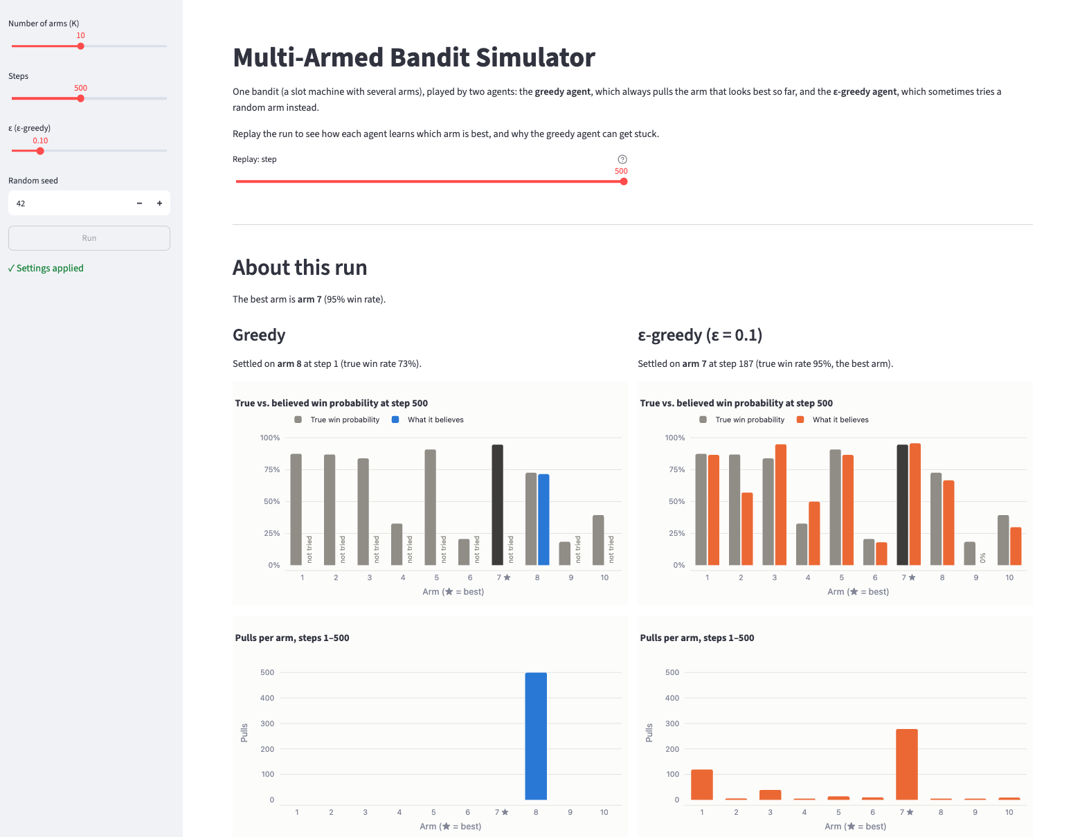
The panel on the left-hand side has the settings of the bandit. You can pick the number of arms, the number of arm pulls (steps) and the probability at which the near-greedy agent will explore (epsilon). Here the seed is used primarily to ensure reproducibility, i.e., making sure that running the bandit with the same settings multiple times always yields the same result. Overall the seed helps control the random aspects of the simulation:

• Setting each arm win probability

• Drawing from the Bernoulli distribution and determine if an arm pull is a win or loss

• Deciding when the near-greedy algorithm will explore

• Picking which arm to explore

• Resolving tie breaks

The agent doesn’t know this but, beforehand we choose the win probability for each arm. This happens before the agent’s first pull and is a random draw from the Uniform Distribution with boundaries between 0.05 and 0.95. The seed ensures we can always reproduce these draws, and the reason why its bounds are between 0.05 and 0.95 is to avoid the scenario of creating an arm that almost always wins or almost always loses.

Then, at every pull of the bandit’s arm, what determines the reward the arm produces is also a random draw. In this case, a random draw from that specific arm’s Bernoulli Distribution, where the result can be either a win (1) or a loss (0).

The seed will also impact when the near-greedy algorithm explores an arm. We set the epsilon to say how often the agent will explore, for instance, 0.1 means it will explore in about 10% of the arm pulls. When it’s time to explore other possibilities rather than sticking to the arm that looks like the highest rewarding arm so far, the agent picks an arm at random, from all the possible arms in the bandit. In the end, the result of this random pick might as well be the arm that looks like the highest rewarding arm, but it was picked at random rather than being a fixed choice like in the greedy algorithm.

Finally, any tie breaks from the agent’s choices are also resolved with a random draw. For instance, in the very first arm pull, the agent doesn’t have any information about estimated expected value for any of the arms of the bandit, so all arms have an estimated expected value of zero. It breaks this tie by picking one arm at random.

With the rationale behind the bandit’s settings out of the way, let’s see the greedy and near-greedy agents in action!

This simulation used the following settings:

• Bandit with 15 arms

• 700 steps/arm pulls for each agent

• Epsilon is set to 0.2, i.e., the near-greedy agent will explore about 20% of the time

• Seed is 42 (because that’s obviously the answer life’s most important questions 🙃)

Greedy Agent

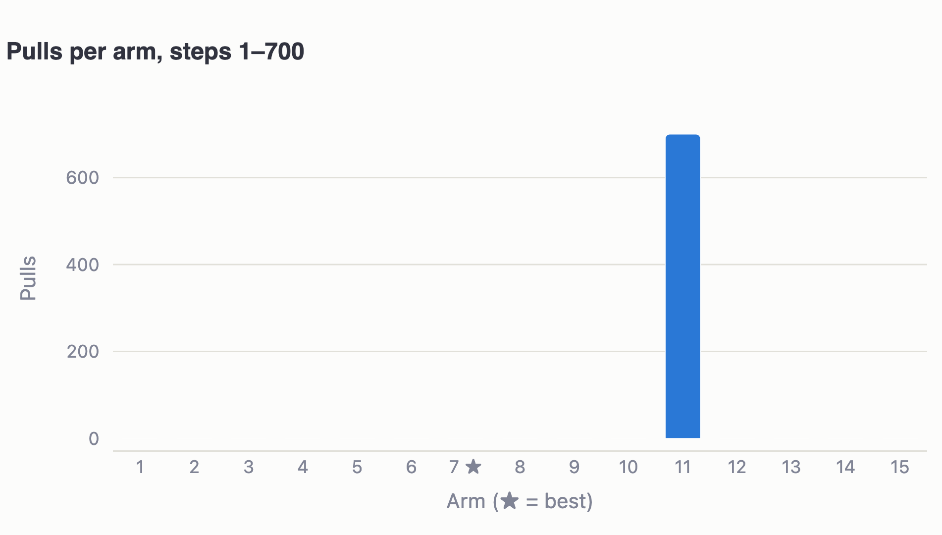
Starting with the Greedy Agent, we can see that as soon as it picked an arm, it stuck to it throughout all 700 pulls. Just doing what’s expected of it.

In this case, the one that looked like the highest rewarding arm was arm 11.

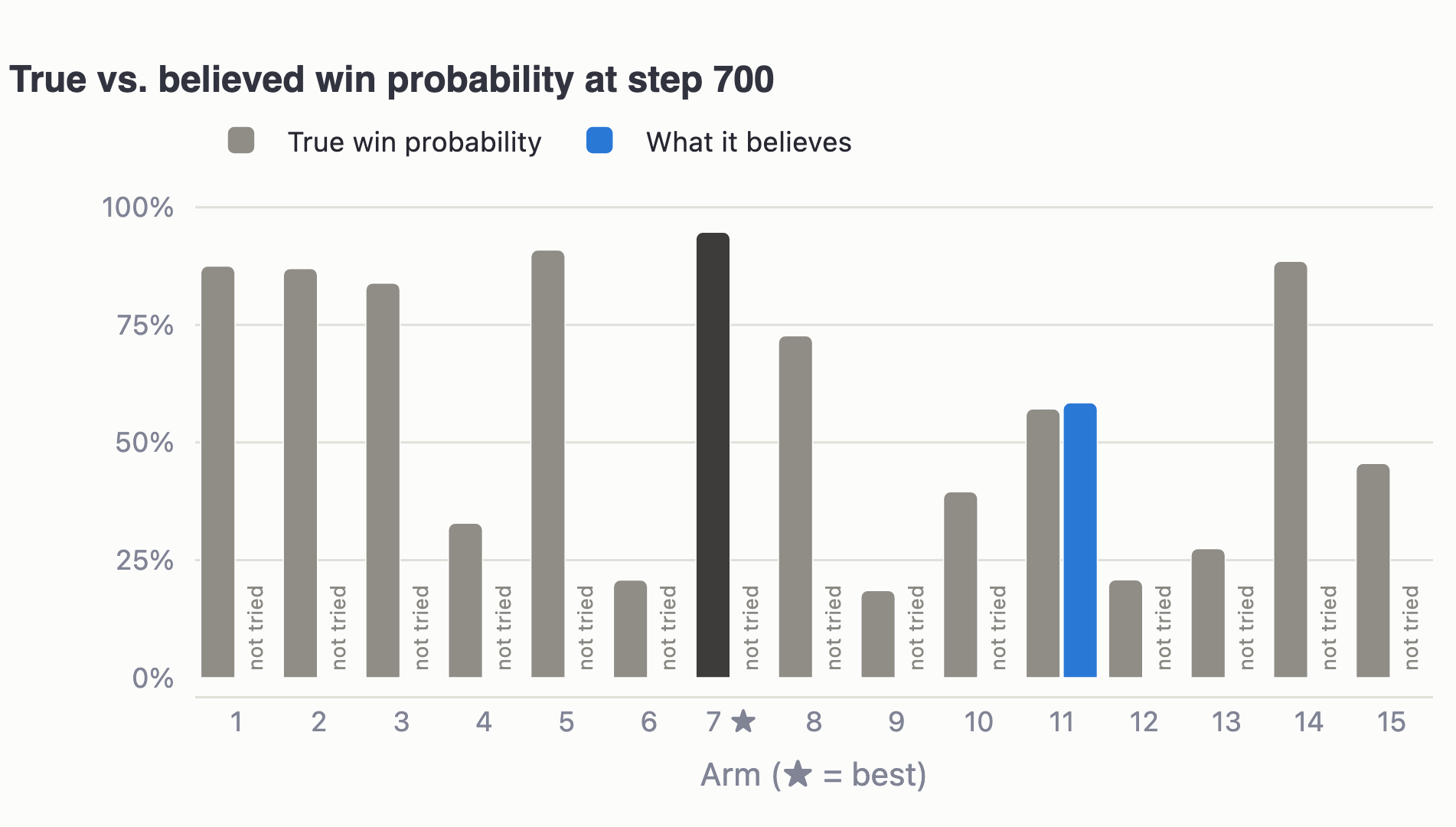
And this becomes very clear, when you see the histogram of pulls per arm across the different 700 steps!

However, going back to the chart with the true win probabilities of each arm, we can see that the greedy agent was quite far from picking the true best arm. It made its choice and stuck to it.

Near-Greedy Agent

Switching to the near-agent, it is set to explore about 20% of the time. And we can immediately see a striking difference compared to the greedy agent.

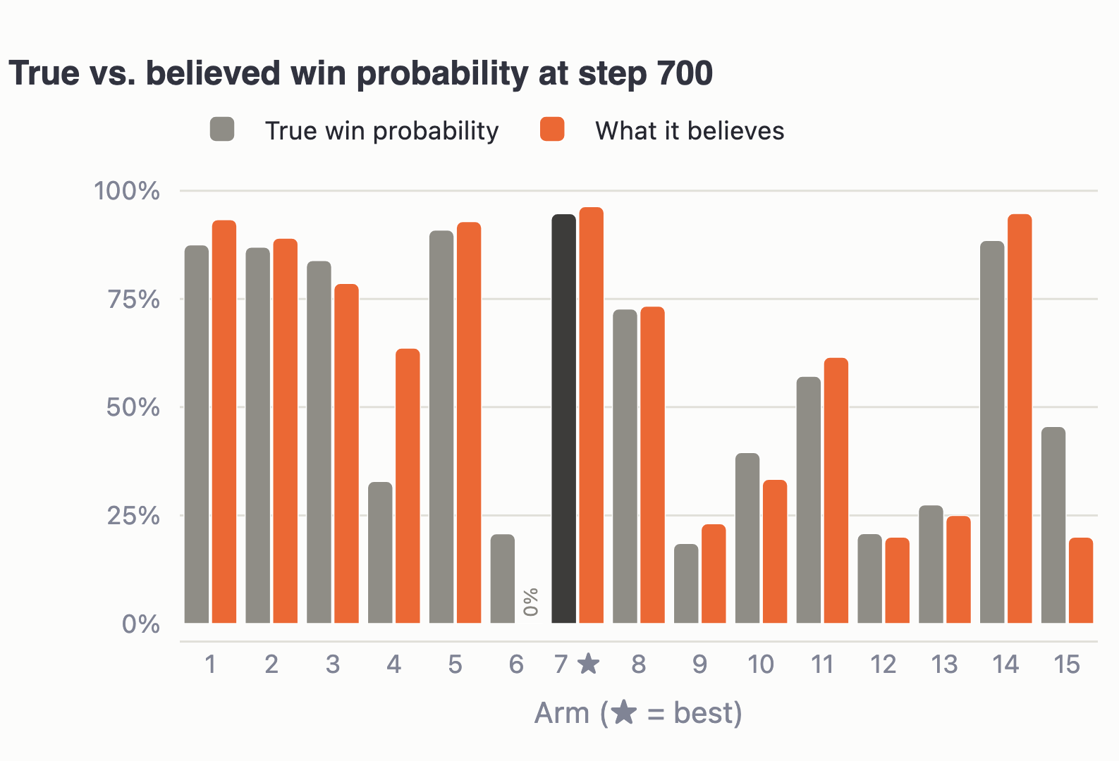
In this case, it settled on arm 7 as the arm that looked like the highest rewarding arm, but we can also see it explore other arms along the way.

Looking at the distribution of pulls per arm, it paints the full picture. It explored a lot but, predominantly, it was pulling arm 7.

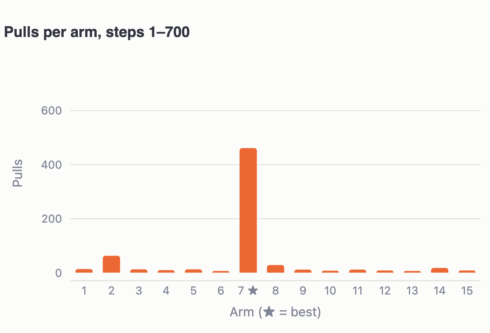
The near-greedy algorithm, proportion-wise, ended up picking the true best arm around 2/3 of the time, you can see its perceived win probability for arm 7 is 96%. It pulled arm 7 in 462 of the 700 arm pulls.

And just based on the agent’s beliefs, arms 1, 5 and 14 were very close calls, with a belief of win probability of 93%, 93% and 95% respectively.

The agent believed arms 1, 5 and 14 had some of the highest estimated value but, in the end, it didn’t pull arms 1, 5 and 14 that often.

This is great! We can clearly see the near-greedy agent exploring the different arms but, is it actually a better strategy?

If we compare the win rate across agents, we can see that, in this case, the greedy agent was lucky when it pulled the first arm, arm 11 because it was a win. But it was greedy and stuck with that choice without exploring and, in the end, it turns out arm 11 was not the true best arm. The near-greedy agent, with its exploratory approach, ended up with the overall highest winning rate.

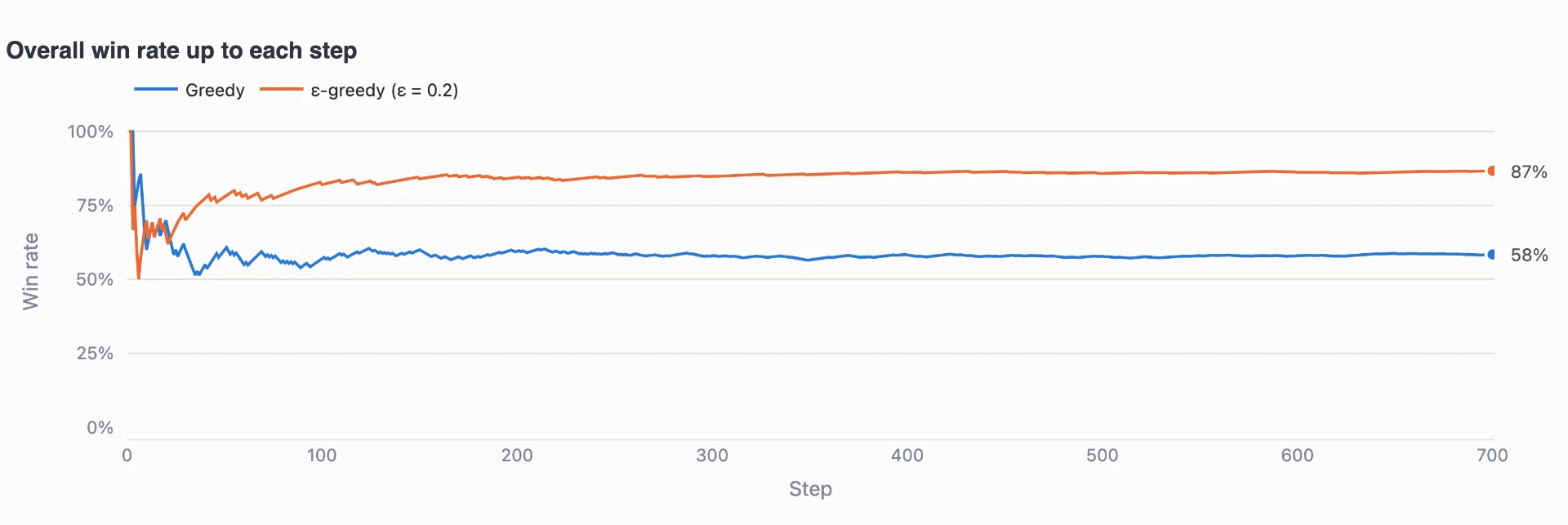
The greedy agent only has an advantage over the near-greedy up to the first 20 arm pulls. After that, in a mix of a sticking with a bad decision by the greedy algorithm and the fact that the near-greedy agent is exploring different options, it ends up with the overall best winning rate. And, in fact, the near-greedy agent found arm 7 by exploring and then stuck to it most of the time, following its beliefs about each arm’s win probability.

This is precisely where we see the trade-off between exploration and exploitation. Look at a close-up that shows the first 32 steps for both agents.

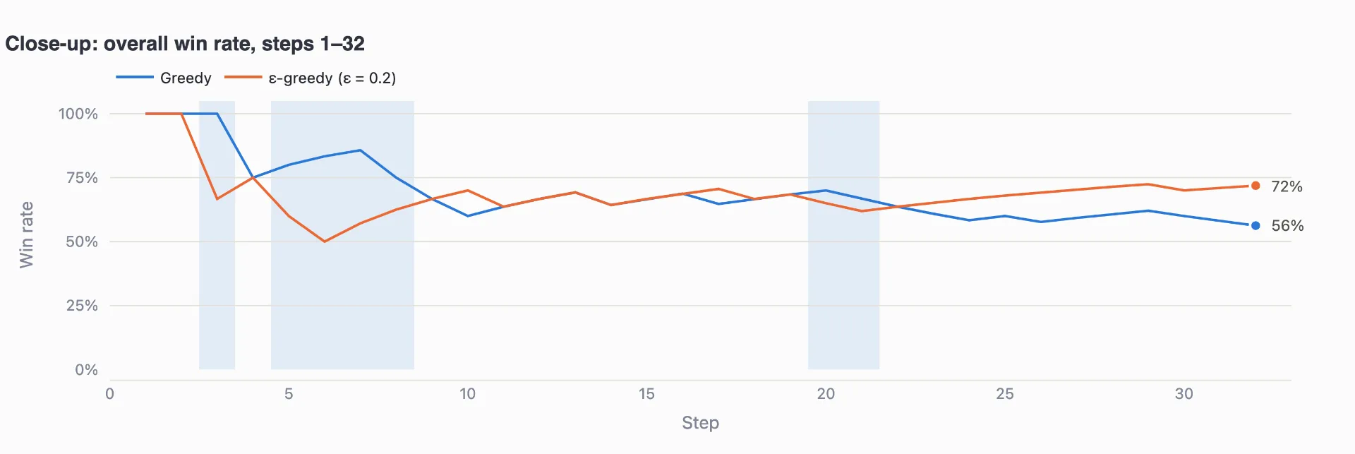
Judging by the see the shaded areas, the near-greedy agent was a bit behind the greedy agent for a while. But, the greedy agent’s initial luck didn’t last long. Later on, the near-greedy agent was able to find the actual highest rewarding arm. In the end, the exploration strategy paid off. After step 21, the near-greedy agent took the lead and the gap widened until the last arm pull. The near-greedy agent ended up with a 87% win rate compared to 58% for the greedy agent.

To see it for yourself, you can use the following Python code.

from pathlib import Pathimport matplotlib.pyplot as pltimport numpy as npfrom matplotlib.ticker import PercentFormatterOUTPUT_DIR = Path("figures")COLORS = {"greedy": "#2a78d6", "epsilon-greedy": "#eb6834"}# Some default settingsdef run_agent(    agent: str = "greedy",    n_arms: int = 10,    steps: int = 250,    epsilon: float = 0.1,    seed: int = 18,) -> dict:    """Let one agent play one bandit and record what it does.    Args:        agent: "greedy" always pulls the arm that looks best so far;            "epsilon-greedy" pulls a random arm with probability `epsilon`.        n_arms: Number of arms on the bandit.        steps: Number of pulls.        epsilon: How often the ε-greedy agent explores (ignored for greedy).        seed: Same seed, same bandit and same run.    Returns:        A dictionary with the agent's name and epsilon, the seed, each arm's        true win probability, and the arm pulled, reward, whether it explored        and all estimates at every step.    """    if agent == "greedy":        epsilon = 0.0    # Random number generator: draws the bandit, the agent's random picks and each win or loss.    rng = np.random.default_rng(seed)    # The bandit: each arm's hidden win probability. The agent never sees these.    win_probs = rng.uniform(0.05, 0.95, size=n_arms)    estimates = np.zeros(n_arms)  # the agent's guess of each arm's win probability    pulls = np.zeros(n_arms, dtype=int)    arms, rewards, explored, history = [], [], [], []    for _ in range(steps):        # 1. Choose: explore a random arm, or exploit the best-looking one.        explore = rng.random() < epsilon        if explore:            arm = rng.integers(n_arms)        else:            best_arms = np.flatnonzero(estimates == estimates.max())            arm = rng.choice(best_arms)  # break ties at random        # 2. Pull: win with that arm's hidden probability.        reward = int(rng.random() < win_probs[arm])        # 3. Update: the estimate becomes the average reward of that arm so far.        pulls[arm] += 1        estimates[arm] += (reward - estimates[arm]) / pulls[arm]        # Record what happened, for the summary and charts. The agent itself doesn't use this.        arms.append(arm)        rewards.append(reward)        explored.append(explore)        history.append(estimates.copy())    return {        "agent": agent,        "epsilon": epsilon,        "seed": seed,        "win_probs": win_probs,        "arms": np.array(arms),        "rewards": np.array(rewards),        "explored": np.array(explored),        "estimates": np.array(history),    }

This snippet creates the agent and the bandit. It returns a dictionary with the agent, the settings and the results of each arm pull. This way you can use the snippet below to print out the summary of the agents run.

def print_summary(result: dict) -> None:    """Print when the agent changed its mind about the best arm, and where it ended up.    Args:        result: What `run_agent` returned.    """    win_probs, estimates = result["win_probs"], result["estimates"]    n_arms, steps = len(win_probs), len(result["arms"])    best_arm = np.argmax(win_probs)    # The arm the agent thinks is best after each step (arm 0 before any pull).    favourite = np.concatenate([[0], estimates.argmax(axis=1)])    changes = np.flatnonzero(favourite[1:] != favourite[:-1]) + 1    settled_arm = favourite[-1]    if result["agent"] == "greedy":        name = "Greedy agent"    else:        name = f"ε-greedy agent (ε = {result['epsilon']:g})"    print(f"{name} · {n_arms} arms · {steps} steps · seed {result['seed']}n")    print("When it changed its mind about the best arm:")    for step in changes:        arm = favourite[step]        estimate = estimates[step - 1, arm]        print(f"  step {step:>4}: arm {arm + 1} now looks best (estimate {estimate:.0%})")    if len(changes) == 0:        print("  never: arm 1 looked best from the start")    pulls = np.bincount(result["arms"], minlength=n_arms)    print("narm  true win prob  estimate  pulls")    for arm in range(n_arms):        star = "★" if arm == best_arm else " "        estimate = f"{estimates[-1, arm]:.0%}" if pulls[arm] else "—"        note = "  ← settled here" if arm == settled_arm else ""        print(f"{arm + 1:>3} {star} {win_probs[arm]:>11.0%}  {estimate:>8}  {pulls[arm]:>5}{note}")    wins = result["rewards"].sum()    when = f"at step {changes[-1]}" if len(changes) else "from the start"    print(f"nWon {wins} of {steps} pulls ({wins / steps:.0%}).", end=" ")    print(f"Explored on {result['explored'].sum()} steps.")    print(        f"Best arm was {best_arm + 1} ({win_probs[best_arm]:.0%}); "        f"the agent settled on arm {settled_arm + 1} {when}.n"    )

These 2 functions just help keep the code organized.

To see the agents in action just need to run:

result_greedy = run_agent("greedy")print_summary(result_greedy)result_e_greedy = run_agent("epsilon-greedy")print_summary(result_e_greedy)

And you’ll see a nice print of each agent’s stats.

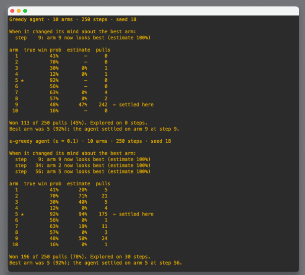
Now, just for illustration purposes, let’s add different settings. You can play around with it as you’d like by passing different parameters to the run_agent function. In this case I only passed the name of the agent I want to run, greedy or epsilon-greedy, i.e., near-greedy. But you can tweak the number of arms, the steps, the epsilon value and the seed.

Just pass it along to the run_agent function like this and see the summary.

result_greedy = run_agent(agent="greedy", seed=32)print_summary(result_greedy)result_e_greedy = run_agent("epsilon-greedy", seed=32)print_summary(result_e_greedy

And you’ll see the agent’s behavior change!

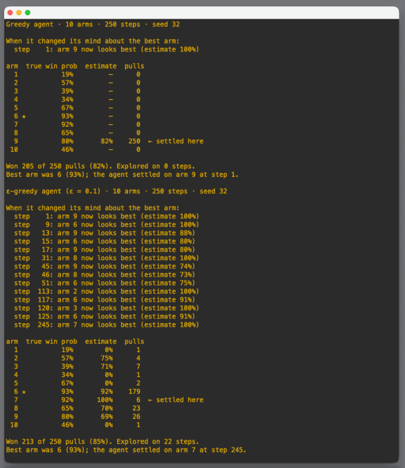
Then, to see the win-rate of each agent, you can take the output of the run_agent function, and use it as an argument to the plot_win_rate function, like this.

def plot_win_rate(result: dict) -> None:    """Save a line chart of the agent's overall win rate up to each step.    Args:        result: What `run_agent` returned.    """    steps = np.arange(1, len(result["rewards"]) + 1)    win_rate = np.cumsum(result["rewards"]) / steps    best = result["win_probs"].max()    fig, ax = plt.subplots(figsize=(8, 4))    ax.plot(steps, win_rate, color=COLORS[result["agent"]], linewidth=2)    ax.axhline(best, color="#3d3c3a", linestyle="--", linewidth=1)    ax.text(1, best + 0.02, f"best arm's win probability ({best:.0%})", fontsize=9)    ax.set_xlabel("Step")    ax.set_ylabel("Win rate so far")    ax.set_ylim(0, 1)    ax.yaxis.set_major_formatter(PercentFormatter(1))    ax.set_title(f"{result['agent']} agent: overall win rate up to each step")    OUTPUT_DIR.mkdir(exist_ok=True)    fig.savefig(OUTPUT_DIR / f"{result['agent']}-win-rate.png", dpi=200, bbox_inches="tight")    plt.close(fig)plot_win_rate(result_greedy)plot_win_rate(result_e_greedy)print(f"Charts saved to {OUTPUT_DIR.resolve()}")

This will output the charts to a folder called figures in the same directory where you’re running the Python script from. But you don’t need to create if beforehand. Notice that in the plot_win_rate function there’s this line.

OUTPUT_DIR.mkdir(exist_ok=True)

It checks if the output directory, in this case figures exists, if not it will create it for you and save the figure with the naming convention [agent-name]-win-rate.png.

Let’s take a look at the greedy agent’s win rate.

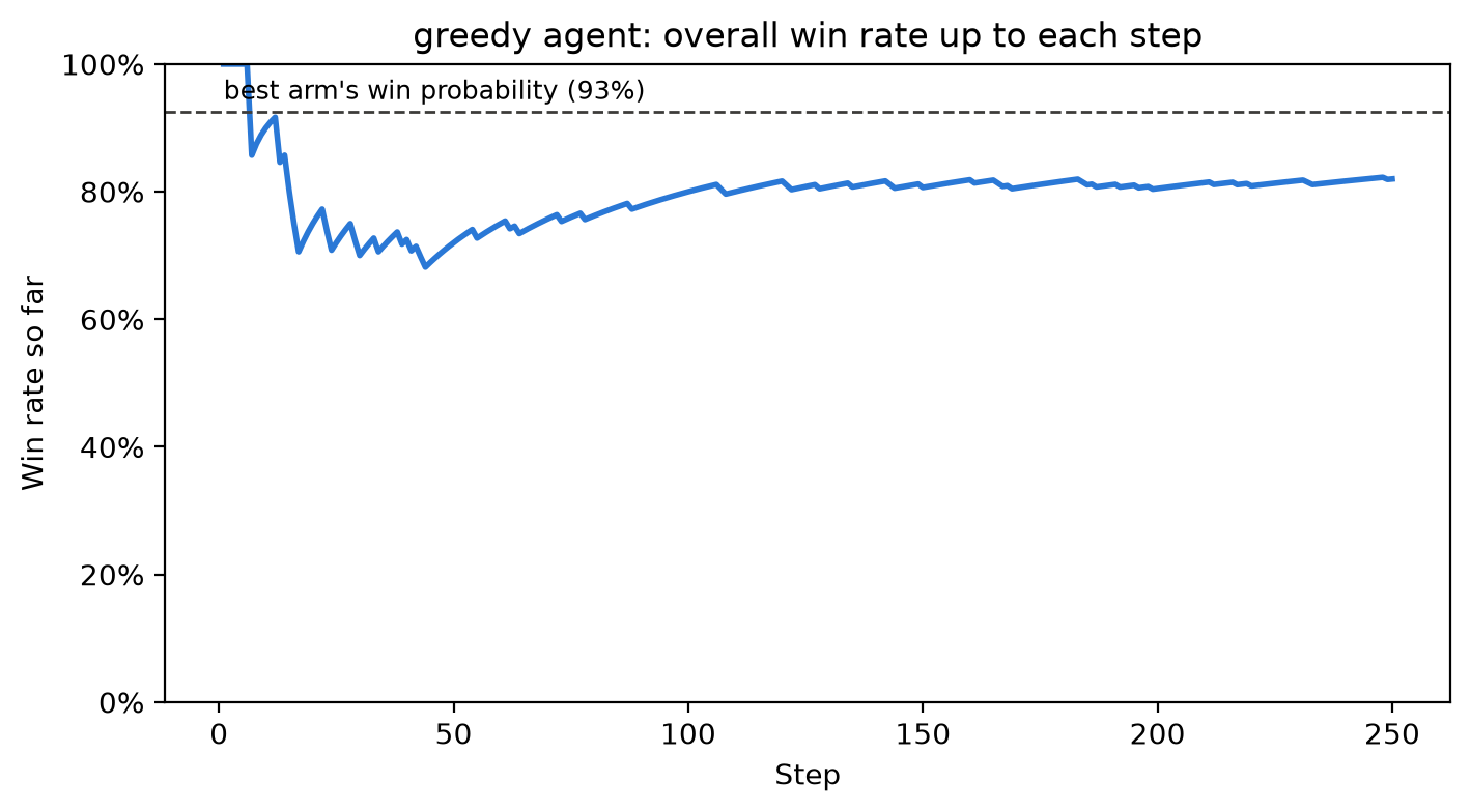
You’ll notice that, in the first pull, the greedy agent pulled arm 9 and determined it had a win rate of 100%. That is because it pulled arm 9, it was a win and, because it had only seen one win so far associated with a total of one pull, it considered the maximum possible win rate, i.e., 100%.

Then, since it is sticking to pulling arm 9, it will pull it over and over again but some of those pulls result in a loss, so its win rate tappers off. In the end, the greedy agent’s win rate is 82%, since in 205 of the 250 pulling arm 9 was a win. It stands a bit below the 93% win rate that would have resulted from always pulling the true best arm, arm 6.

The near-greedy agent, on the other hand, ends up exploring quite a bit.

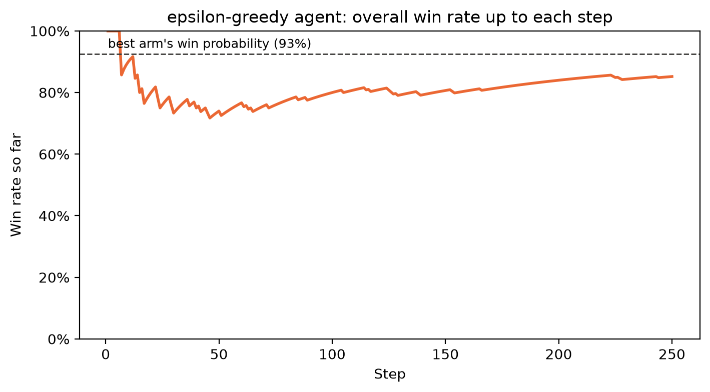
The first 6 pulls it observes a 100% win rate because, although it didn’t pull the true best arm, arm 6, it got 6 wins in a row. So, 6 wins in 6 pulls sets the 100% win rate. Then it has a loss on the seventh pull, wins again on the 8th arm pull and goes on to explore pulling different arms starting on the 9th pull.

The near-greedy agent was quite close to settling on the true best arm. From its pulls it ended believing the best arm was arm 7, while the true best arm was 6.

And, although below the best arm’s true win probability of 93% it obtained an overall win rate of 85%. Since in 213 of the 250 pull it got a win.

It’s very interesting to see how both agents perform in such a different way. And, in the end, the near-greedy agent, due to the way it explored the different arms available to pull, was able to surpass the greedy agent.

Conclusion

There are many more Reinforcement Learning algorithms, this article only scratched the surface.

We’ve only touched on one type of problem within Reinforcement Learning, the Multi-Arm Bandit, but this is a currently active research area with many tangible applications. For instance, your favorite coding agent certainly uses some flavor of Reinforcement Learning to fine-tune its underlying Large-Language Model[7].

I hope this article as sparked your curiosity about Reinforcement Learning and that it can inspire you to learn more.

Thanks for reading!

References

1. https://cloud.google.com/discover/what-is-reinforcement-learning

2. R. S. Sutton and A. G. Barto, Reinforcement Learning: An Introduction, 2nd ed. Cambridge, MA, USA: MIT Press, 2018.

3. N. Hirose, D. Shah, K. Stachowicz, A. Sridhar, and S. Levine, “SELFI: Autonomous self-improvement with reinforcement learning for social navigation,” arXiv preprint arXiv:2403.00991, 2024.

4. Y. Liu et al., “A review of reinforcement learning for natural language processing, and applications in healthcare,” arXiv preprint arXiv:2310.18354, 2023.

5. MIT 6.S191: Reinforcement Learning

6. A. Slivkins, “Introduction to multi-armed bandits,” arXiv preprint arXiv:1904.07272, 2019.

7. L. Ouyang et al., “Training language models to follow instructions with human feedback,” arXiv preprint arXiv:2203.02155, 2022.