What OpenAI’s 719 Math Papers Mean for Data Science

Scott Aaronson pictures a hunter-gatherer who has spent a lifetime learning to survive in a rainforest, only to find a resort opening next door, complete with heated pools and Airbnbs. The hunter-gatherer adjusts his career plans:

“alright fine, so now my new job is to run wilderness retreats for the tourists, or something.”

That is Aaronson’s analogy for the mood in mathematics after OpenAI’s release. He tells it in The Mathocalypse.

On 6 October 2026, OpenAI released a collection that now contains 719 papers in 372 groups of related results, produced by an unreleased internal model. Some concern familiar data-science tasks: matching messy text, choosing representative observations, generating comparison data and fitting models. A proof can establish that a better method is possible long before anyone has an implementation worth using.

Joe Halliwell’s look at the release’s practical consequences follows several results towards everyday applications. The examples here show how our choices about accuracy, distance and randomness determine the computation, storage and data we need.

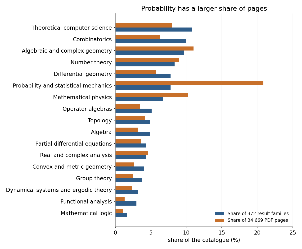
Computer science leads in families; probability leads in pages

OpenAI calls each group of related results a result family. A family may include several connected results or different ways of proving one result. Of the 372 families, 205 contain one paper and 301 contain no more than two. The largest contains fourteen.¹

The release covers seventeen disciplines. Theoretical computer science has the most families, with 40, about 11% of the total. Count pages instead, and probability and statistical mechanics takes the largest share: 29 families contain 105 papers and 7,232 pages, about 21% of all pages.

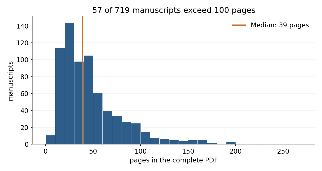
The complete collection runs to 34,669 pages. The median paper is 39 pages long, and 57 exceed a hundred. Reading one PDF a day would take almost two years, assuming a 262-page paper counts as a normal Tuesday.

Some results relevant to data science sit elsewhere in the catalogue: the result about compressing feature vectors below is filed under convex and metric geometry.

Comparing long strings gets a better speed guarantee

Consider two entries in a customer table: Jon Smith and John Smyth. A strict text match treats them as strangers. To compare the spellings, count the fewest single-character insertions, deletions and replacements needed to turn one into the other. Here, insert an h and replace i with y: two edits. This count is edit distance, a useful ingredient in matching records whose text differs slightly.

The standard exact calculation builds a grid, with positions in one string along the rows and positions in the other along the columns. Each cell records the cheapest way to match the text up to those positions. Two strings of 10,000 characters give about 100 million cells. Double both lengths and the grid becomes four times larger.

The new edit-distance paper claims a method whose average work grows almost in proportion to the total text length, for any fixed percentage error allowance. Choose 1%: if the true distance is 100, a successful estimate is 100 or 101. The method uses randomness and promises an estimate within the allowance at least two times out of three.² Combining such a small error allowance with almost-linear growth improves on the earlier guarantees discussed in the paper.

The published recipe still uses the exact grid calculation below an enormous input-size threshold. Getting its better growth rate to pay off at lengths we can actually store is further work. Its output is a score, useful for ranking candidate matches; producing the actual list of edits would take another step.

A better clustering guarantee limits the cost of a bad answer

Suppose you have thousands of support tickets and a colleague willing to read six. The colleague’s willingness is the scarce resource. You want those six tickets to represent the archive as closely as possible.

Represent each ticket as a feature vector, with similar tickets close together. Choose some actual tickets and add up every ticket’s distance to its nearest chosen example. A smaller total means better coverage under your chosen distance measure.

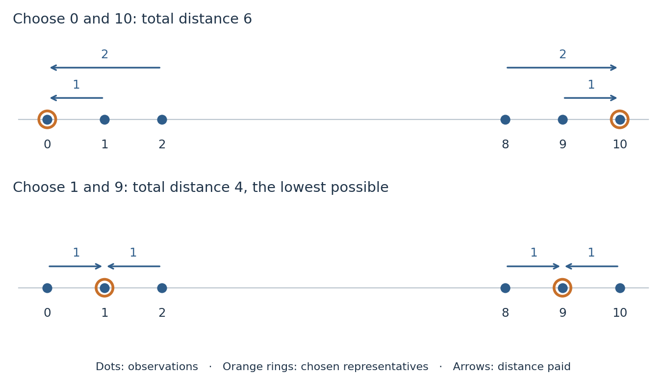
For six points on a line, 0, 1, 2, 8, 9 and 10, choosing representatives 0 and 10 gives a total distance of 6. Choosing 1 and 9 gives 4: each serves itself and two neighbours one unit away.

Choosing k actual observations this way is called k-medoids. KMeans can put a centre between observations, which is reasonable geometry but awkward when your colleague asks to read the ticket. The broader k-median problem allows a separate list of candidate locations, such as depots serving customers.

The number of possible selections soon makes checking them all expensive. OpenAI’s k-median paper claims a tighter promise for its algorithm: if the best selection costs 100, the previous general guarantee allowed roughly 200; the new ceiling approaches 173.6.³This approximation guarantee covers every allowed dataset. Distances must obey the rule that a detour through a third point cannot be shorter than the direct journey.

The algorithm starts with an easier depot plan that permits partial openings. Six locations serve customer pairs AB, BC, AC, DE, EF and DF. Each customer is distance 1 from its two associated locations and distance 3 from the rest. We can open three depots. Opening all six halfway gives each customer half its service from each nearby location: cost 1 per customer, 6 overall. Six half-open depots fit the budget, though the building contractor may want further instructions.⁴

Whole depots cost at least 8: choosing AB, BC and DE leaves F travelling distance 3 while everyone else travels 1. Giving all six customers a nearby depot needs four openings. The code prepared for this post confirms both optima, 6 and 8.

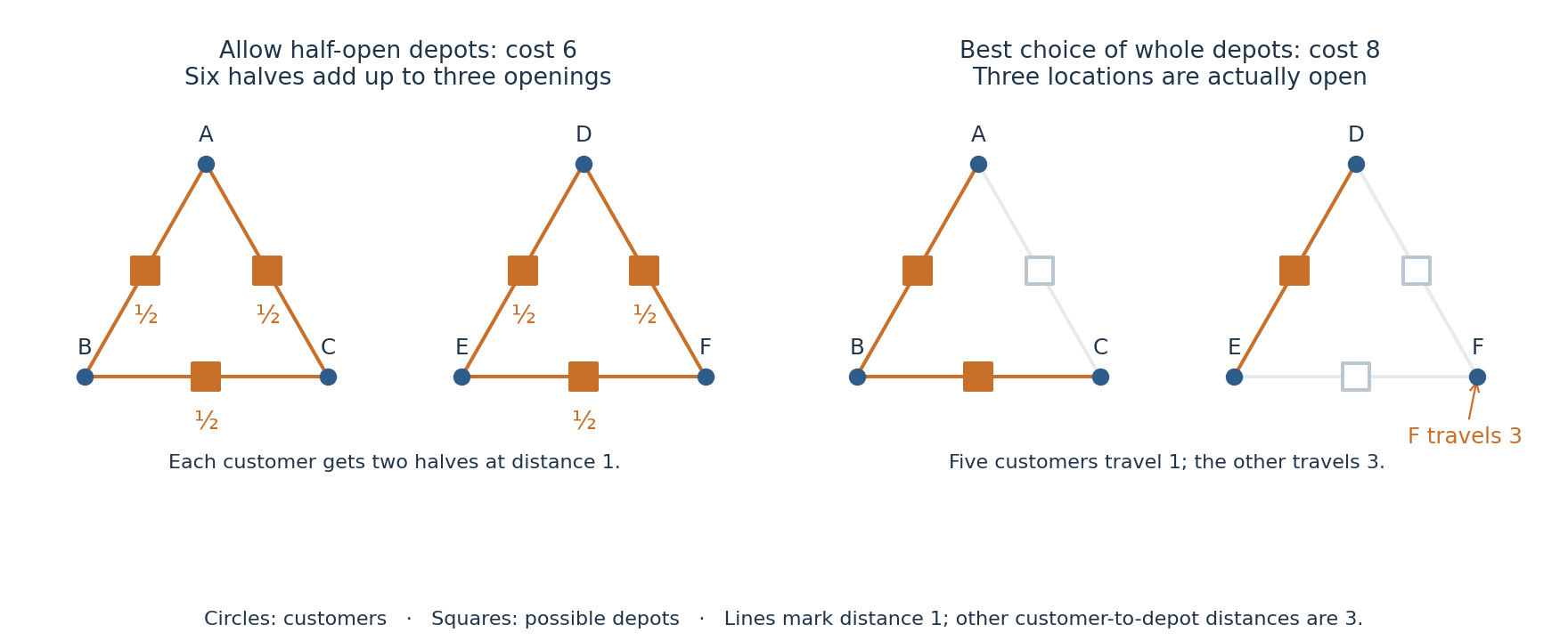
Allowing partial openings can only make the best plan cheaper. Converting that optimistic plan to whole depots is called rounding. Controlling the extra cost helps prove a guarantee: a solution costing at most twice the optimistic plan also costs at most twice the best real plan.

I wanted to benchmark the complete algorithm. Following its published recipe literally, even for a looser guarantee, divides one fully open location into more than 6 × 10²⁸ tiny pieces. Touching each once at a hypothetical trillion pieces per second would take nearly two billion years.⁵ A practical implementation would need to avoid creating each piece separately.

Familiar clustering methods already do well on the small test

The existing benchmark compares familiar methods on fifteen small problems. An optimisation solver established their best costs within its numerical tolerances.⁶ A common shortcut swaps representatives whenever that lowers the cost, stopping when no single swap helps. A larger rearrangement might still do better.

Two versions of this swapping method each matched the best cost on fourteen of fifteen problems; their largest misses were 0.8% and 0.3%. Replacing each KMeans centre with its nearest actual observation was at worst 4.2% above the best cost.

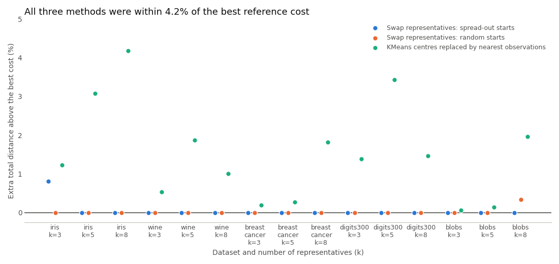
These fairly friendly datasets leave little room to improve answer quality. Comparing OpenAI’s algorithm will need a working implementation, harder examples and timings.

Random tables can preserve every row and column total

Suppose you have counts of tea and coffee sales in two regions:

To study the regional pattern, you could generate comparison tables that keep both sets of totals fixed. Each region must still sell 50 drinks, with 60 teas and 40 coffees overall. Giving each region 30 teas and 20 coffees is one alternative. Moving a sale between cells forces compensating changes elsewhere.

This is a contingency table: counts split by two categories. One way to randomise it gives every table satisfying the totals an equal chance. In our tiny example, choosing North’s tea count determines all three other cells. Larger tables leave many interdependent choices.

The new sampling paper claims a method that produces exactly this uniform distribution for arbitrary compatible totals, with both the number of rows and columns free to grow. Earlier running-time guarantees described in its introduction required restrictions, such as a fixed number of rows. The new guarantee covers very uneven totals too.⁷

That provides a way to construct random data while retaining chosen features of the original. The probability model matters: giving every table equal weight differs from shuffling individual sales records, which can produce some tables in more ways than others. I would decide which comparison fits the analysis before choosing a sampler.

The paper’s running-time bound is an average over random choices, with deliberately large powers in the formula. Turning that guarantee into a useful data-generation tool still needs implementation and measurement.

Limited memory can force a learner to use more data

Imagine fitting a model as rows arrive, without keeping the dataset. Useful information from old rows must survive in the learner’s stored state.

Suppose two unknown numbers, a and b, have sum 3 and difference 1. Together these observations give a = 2 and b = 1. Forget the sum, and both (2, 1) and (2.5, 1.5) fit the remaining information. More computation cannot recover the distinction; another observation could.

With a long stream and a fixed memory budget, the learner must choose what survives. The memory-and-precision paper studies normally distributed inputs and labels calculated from the true weights with no noise. Memory includes the bits needed to store numbers accurately.

A fixed-size summary has finitely many states, so different histories can leave identical stored information. Finer estimates require more distinctions between possible weights. Keeping extra digits can preserve those distinctions, but uses more memory.

For any summary within its stated memory budget, the paper bounds the sample budget the learner must be allowed. That lower limit grows with the number of times you halve the permitted error.⁸ Computation between observations is unlimited.

This connects how much data to collect with how much information to retain. Even the theorem’s very considerate dataset, with no wrong labels at all, cannot remove that trade-off.

Accepting a little distance error can save many coordinates

A feature vector is a row of numbers. To find similar observations, you may need the distances between rows more than every original coordinate.

Observations at (0, 0), (3, 4) and (6, 8) have distances 5, 5 and 10. Store them as 0, 5 and 10 on one axis, and those distances survive using one number per observation. This dimension reduction is easy because the points already lie on a line.

Existing methods preserve ordinary straight-line distances approximately in much more complicated datasets. The new paper concerns other distance rules. One adds fourth powers of coordinate differences and takes a fourth root, instead of using squares and a square root. From (0, 0), the distance to (1, 1) becomes about 1.19 rather than 1.41, while (1, 0) remains distance 1. The rule changes what counts as similar.

Using the chosen rule before and after compression, preserving distances exactly can require a number of coordinates that grows as the square of the number of observations. Allow a fixed percentage of error, and the paper’s bound eventually grows more slowly than the square root of that number.⁹

A 10% allowance means that, after multiplying every new distance by the same number, no distance shrinks and none grows by more than 10%. Nearest neighbours can still swap order: distances 100 and 101 could become 110 and 101.

The proof establishes that such a representation exists for the supplied points. An efficient construction and handling later observations remain further work.

The speed records use different ways of counting work

The speed claims for three familiar operations depend on how work is counted.

The sampling result uses the accounting of a report that counts database queries and regards all the Python afterwards as a personal matter. Ten calls can still be followed by a day processing their responses.

A paper on moving one distribution onto another finds a weaker stability guarantee than researchers had conjectured: similar target distributions can require less similar movements of individual points.¹³ For a data-alignment pipeline, I would check how observations move as well as how closely the distributions match.

Computer-checked proofs still need a careful reading of the claim

A proof checker is a program that checks whether an argument’s steps establish a precisely written statement from its assumptions. Lean is one such program, and journalist Kevin Hartnett tells the story of its development in The Proof in the Code.

OpenAI reports computer-checked proofs for the main results in 300 of its 719 papers, about 42%. These checks cover specific results within each paper. For example, the quasi-Riemann paper’s computer-checked proof covers its main result, but leaves out the further conclusions the paper draws from it.

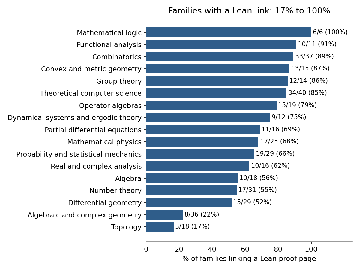
The catalogue lets us make a different count: groups of related papers that link to a page describing a Lean proof. All six mathematical-logic families have such a link, compared with three of eighteen topology families. Overall it is 242 of 372 families, about 65%. Each scope page specifies which results its proof covers.

The repository history records three withdrawn papers: a sign error invalidated one construction and two papers that depended on it.

Experts are finding ideas worth learning in the unfamiliar proofs

Dana Moshkovitz had spent roughly two decades working on Unique Games, a problem connected to limits on how closely algorithms can approach the best answer. Her first reaction to the new proof was confusion. Aaronson quoted her complaints about unexplained steps and confusing citations, and her description of the construction as “some alien craziness”.

She asked Astra, an AI assistant, to explain the proof interactively. By the following day, Aaronson reported that she largely understood the proof and was amazed by its new ideas.

In the comments, Jonathan Baxter suggests that a model may treat an argument scattered across ten pages as equivalent to a clearly organised version. Think of inheriting a notebook that produces the right answer, once you discover that cell 47 has to run before cell 12. Getting it to work and understanding it well enough to change it are separate jobs.

Aaronson compares the model to a junior researcher with extraordinary breadth of knowledge, the ability to connect techniques across fields and unusual persistence. Moshkovitz also emphasises that the new results build on human communities and earlier work.

I think this is a reason to study the release even before its algorithms are practical. A method that looks unwieldy in the general proof may contain an idea we can adapt to a narrower task. Understanding the reasoning is what would let us identify that idea and check whether our adaptation still works.

There is another consequence of making these results public. ⁠Hugging Face has already converted 369 of OpenAI’s mathematical challenges into reinforcement-learning environments, where models attempt formal proofs and receive feedback from a verifier. This is not conventional model distillation: no access to OpenAI’s weights or internal reasoning is required. Instead, it offers a form of capability transfer, allowing smaller open models to train against mathematical problems and verification infrastructure derived from frontier research. The current verifier is limited, however, and can reject mathematically equivalent proofs expressed differently. The interesting question is whether this training generalises beyond reproducing known results. Could a 7B-parameter model, ultimately running on commodity hardware, use what it has learned to make a genuinely new mathematical discovery? Solving a Millennium Prize Problem would be an extraordinary demonstration, although there is still an enormous distance between these training environments and that ambition.

For the k-median paper, the next useful step is to turn its partial-opening plan into a manageable implementation, identify which promises survive any simplification, and compare both answer quality and running time.

Disclaimer: This was an informal, curiosity-driven project undertaken in my personal time. The views expressed here are my own and do not represent those of my employer or any affiliated organisation. The content is based on personal experience and reflection, and should not be taken as professional or academic advice.

···

1. Counts use the groupings, subject labels and PDFs in repository snapshot fd4aeeb, checked on 10 October 2026. All 719 PDFs were counted, including references and appendices. Lean coverage counts groups with a link to a page describing a formal proof.↩︎

2. Each inserted, deleted or replaced character costs one. The accuracy allowance stays fixed as the strings get longer. Average work means an average over the algorithm’s random choices, even for the hardest input pair of a given length; it includes reading the strings and the rest of the computation. The result estimates the distance between a pair of strings, so finding candidate pairs in a large table remains a separate job.↩︎

3. The factor is approximately 1.736 plus a small positive allowance. Choosing an allowance of 0.004 gives a factor below 1.74; smaller allowances may require much more computation. The earlier roughly-two guarantee held with high probability over random choices; the new algorithm uses no randomness. Both guarantees concern algorithms whose work grows at most as a fixed power of the input size. The guarantee covers the general depot problem, including cases where candidate depots and customers occupy different locations.↩︎

4. Customers are distance 2 from one another, as are depot locations. These distances obey the rule that going via a third point cannot shorten a journey. Each customer must contribute at least 1, so the partial-opening total of 6 is as low as possible. All twenty choices of three whole depots were checked.↩︎

5. The calculation follows the proof’s instructions for a guarantee of about 1.836 times the best cost. They require at least 6.1 × 10²⁸ pieces. Dividing by a hypothetical trillion pieces per second, then by the seconds in a year, gives about 1.94 billion years.↩︎

6. The benchmark compares the three existing methods shown in the chart. It uses iris, wine, breast cancer, 300 handwritten-digit examples and 300 synthetic points, each with 3, 5 and 8 representatives. Features were put on a common scale. The solver found the best cost for all fifteen cases within its numerical tolerances. Each swapping method kept the best of ten starts. Its largest gap was 0.8% with spread-out starts and 0.3% with random starts.↩︎

7. Counts are nonnegative whole numbers, with no forbidden cells or extra cell limits. Expected work is polynomial in the row and column counts and the number of binary digits needed for the totals. A very rare branch does exhaustive computation, so the bound applies on average, not to every run.↩︎

8. Memory is measured in bits, so storing more digits uses more of the budget. The theorem allows memory proportional to the square of the number of features. It assumes many features, exact labels and normally distributed inputs. The learner must estimate the direction of randomly chosen weights, with at least a two-thirds chance of success. Error is measured as the angle between the learned and true directions.↩︎

9. These distance rules add powers of absolute coordinate differences, then take the corresponding root. The power can be any fixed finite number greater than 1. Ordinary straight-line distance uses power 2 and already has a stronger known result. The new representation can reshape the data in complicated ways; it need not be a straight projection.↩︎

10. The paper brings the growth exponent arbitrarily close to 2.25, down from about 2.37. The exponent describes how the work scales as matrices get larger; constant multipliers still matter for any actual calculation.↩︎

11. Ignoring constant multipliers, the old and new formulas differ by only about four parts in ten trillion at 2⁶⁴ inputs. The paper assumes arithmetic without rounding and reports enormous constant multipliers. The algorithm is given an exact complex number representing a specified rotation. Multipliers and intermediate values have no size limit.↩︎

12. The paper works with a smooth, bowl-shaped function: the negative log-density plus a constant. In every direction, the rate at which its slope changes must stay between 1 and 2. The bottom of the bowl is supplied. Each request returns the function’s exact value and gradient. The samples must match the target within a fixed error tolerance.↩︎

13. The starting distribution is uniform over a bounded region in at least two dimensions. The straight path between any two points in the region must stay inside it. The target also stays within a fixed bounded region. A target with just three possible locations is enough to show why the stronger proposed guarantee fails.↩︎