A Beginner’s Guide to World Models

Intro

In Machine Learning, a World Model is a system that builds an internal representation of an environment and predicts how that environment changes over time in response to actions. Simply put, it’s an AI model that simulates the world’s dynamics (i.e. physics, object interactions, causality). These days, World Models are being used to power robots, autonomous driving, and interactive video generation because they allow an AI to “think before it acts” by running mental simulations of reality.

Early ideas date to the 1990s, when German researchers designed Recurrent Neural Networks that predict future states from observations and used those predictions to train agents without constant real-world trial and error. Then, in 2022, Yann LeCun revived the idea of autonomous machine intelligence, saying that intelligence requires predictive models of the world rather than pure pattern matching. The first World Model proposed by LeCun was the Joint Embedding Predictive Architecture (JEPA) with the idea that giving an internal representation of how the world functions to a self-supervised model, it could improve its results. The key idea is that the AI learns how the physical environment (the “world”) works by predicting abstract concepts in a continuous space, rather than guessing the next token (e.g. pixel or word). For this reason, JEPA is very different from Transformer architectures, and it’s considered the foundation for World Models.

In 2024, Google introduced its World Model Genie, a research prototype that lets you create and explore infinitely diverse worlds. California’s autonomous taxi Waymo adopted Google’s Genie to create its own specialized model for self-driving simulation (Waymo World Model).

State of the Art

In 2026, the startup World Labs released Marble, an AI with “spatial intelligence” that can create interactive and explorable 3D environments from text prompts. Similarly, Alibaba launched its World Model Happy Oyster, designed for world-building based on text and image prompts. Then, the latest World Model was released in June 2026 by Nvidia: Cosmos, a family of open-weight models that combine physical reasoning, world simulation, and action generation. Those three World Models represent the current state-of-the-art.

For example, I’ll write a prompt on Alibaba’s Happy Oyster to generate an environment.

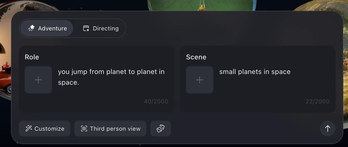
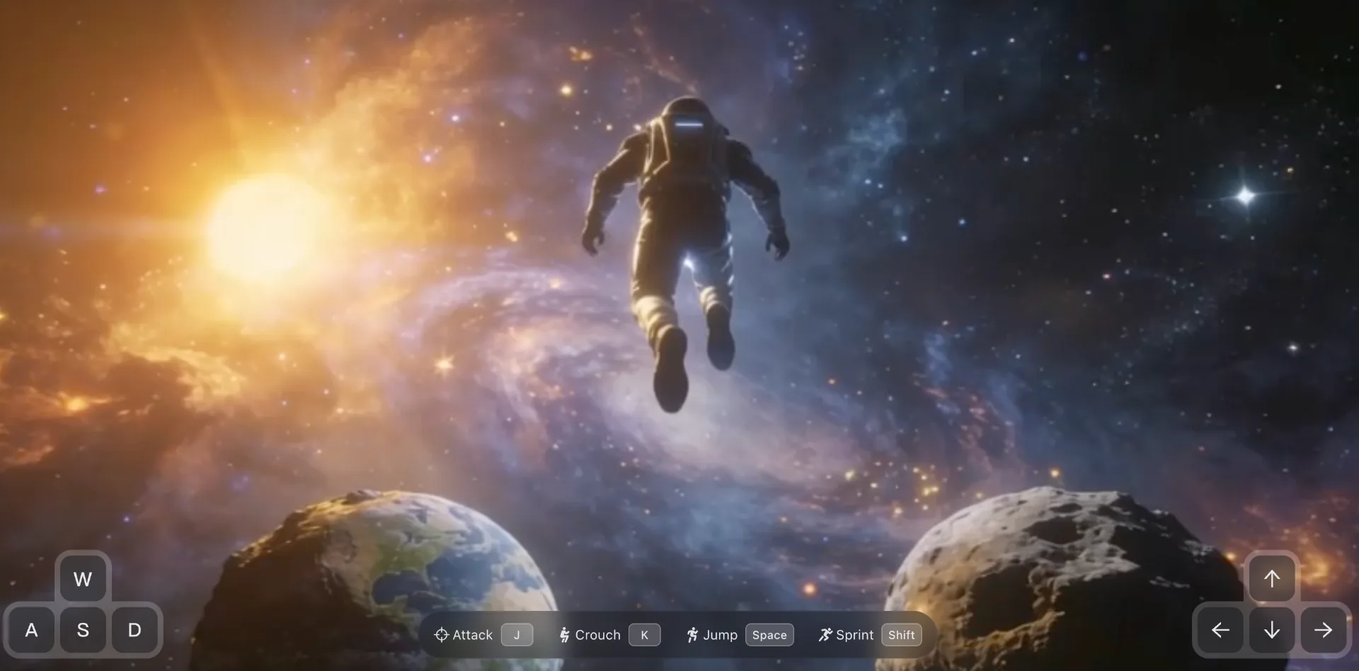
And just from this simple prompt, the model creates a confined 3D world that you can explore for a limited time (2 min) in a sort of video game style.

Architectures

Basically, World Models are systems that build an internal simulation of an environment to predict its future states. They can be categorized into four architectures:

• Joint Embedding Predictive Architectures (JEPA) eliminate the need for generative decoders and prevent the model from wasting computational power on unpredictable background details (like flickering leaves) by forcing it to focus only on large-scale physical dynamics.

• Recurrent Stochastic State Models (RSSM) process sequential data by breaking it into a belief state (long-term memory) and a stochastic state (to capture environmental randomness and uncertainty).

  • Use-case: open-source project Dreamer.

• Tree-Search Models, instead of predicting what the next frame looks like, predict the next hidden state, the action value, and the immediate reward, integrating a Monte Carlo Tree Search to plan ahead.

  • Use-case: Google’s MuZero.

• Generative Foundation Simulators use autoregressive Diffusion Transformers trained on massive internet-scale video datasets, and act as real-time generative video game engines. They take text, image, or action prompts and generate temporally consistent, physically plausible photorealistic future frames.

  • Use-case: Google’s Genie and Nvidia’s Cosmos.

Build a World Model

The easiest and most accessible type of World Model is SGF (Simple, Good, Fast). It’s a simplified non-recurrent latent dynamics model where spatio-temporal data is compressed into a hidden layer (latent space) without using traditional recurrent loops (like LSTMs). I’m going to build a World Model inspired by the SGF approach, combined with the general latent-dynamics architecture introduced in this paper, which adds a decoder layer to reconstruct the prediction as an image.

For the environment, let’s use the Atari game BattleZone (pip install ale-py) and the famous Gymnasium library (pip install gymnasium).

import gymnasium as gymimport ale_pyenv = gym.make("ALE/BattleZone-v5")N_ACTIONS = env.action_space.nprint("Actions:", N_ACTIONS)

The environment is a discrete space of 18 possible actions (go right, go left, attack…), therefore the model will have to learn meaningful spatial dynamics: your tank moves, enemies appear in different directions, projectiles travel, and the camera changes.

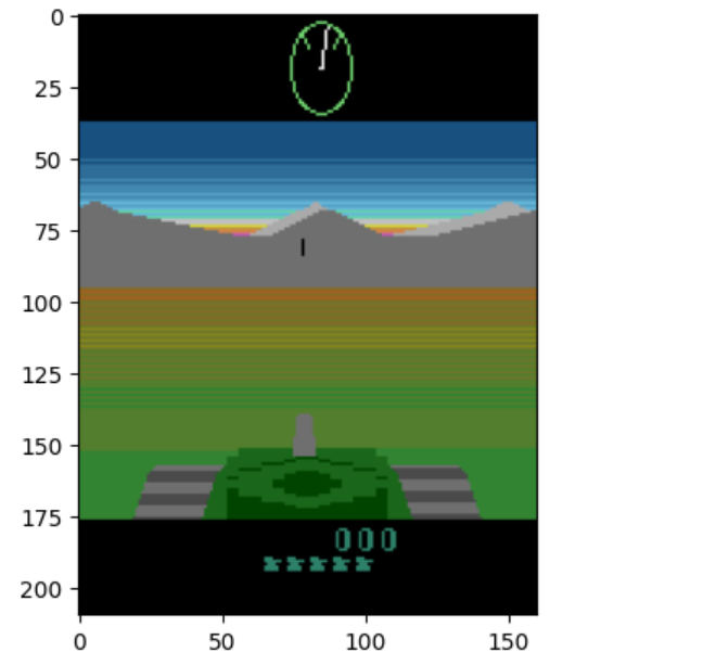
import matplotlib.pyplot as pltobs, _ = env.reset()plt.imshow(obs)plt.show()

I will build a World Model Neural Network using PyTorch (pip install torch). The input data is Atari RGB pictures (210x160x3) with raw pixel values (0-255). The first step is cleaning and reshaping the data into a small grayscale tensor (1x64x64) with normalized values (0-1), so the Neural Network can digest it efficiently.

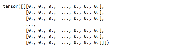
import torchimport torch.nn.functional as FIMAGE_SIZE = 64def preprocess(obs):    """    Atari RGB image    -> grayscale    -> 64x64    -> [0,1]    """    x = torch.tensor(obs, dtype=torch.float32,)    # HWC -> CHW    x = x.permute(2, 0, 1)    # RGB -> grayscale    x = x.mean(dim=0, keepdim=True,)    # 64x64    x = F.interpolate(        x.unsqueeze(0),        size=(IMAGE_SIZE, IMAGE_SIZE),        mode="bilinear",        align_corners=False,    )    return x.squeeze(0) / 255.0obs, _ = env.reset()preprocess(obs) 

Now that we can process data, we should start our data collection by building a memory of the game’s experiences. The collection loop runs the game using random actions and stores each example (obs, action, next_obs) in the Replay buffer. So after this loop, we have a dataset of how the environment behaves: “I saw this image → I took this action → then I saw this next image”.

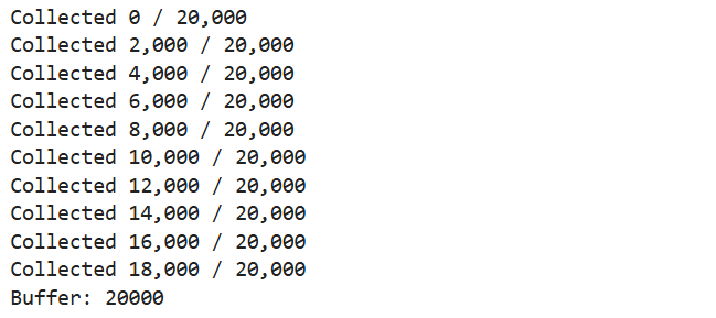
import randomfrom collections import dequeBUFFER_SIZE = 20_000class ReplayBuffer:    def __init__(self, capacity):        self.buffer = deque(maxlen=capacity)    def add(self, obs, action, next_obs):        self.buffer.append((obs, action, next_obs))    def sample(self, batch_size):        batch = random.sample(self.buffer, batch_size)        obs, actions, next_obs = zip(*batch)        return (            torch.stack(obs),            torch.tensor(actions, dtype=torch.long),            torch.stack(next_obs)        )    def __len__(self):        return len(self.buffer)buffer = ReplayBuffer(BUFFER_SIZE)# PLAY RANDOM TO COLLECT DATA INTO THE BUFFERobs, _ = env.reset()for step in range(BUFFER_SIZE):    action = env.action_space.sample() #random action    next_obs, reward, terminated, truncated, _ = env.step(action)    buffer.add(        preprocess(obs),        action,        preprocess(next_obs),    )    obs = next_obs        if terminated or truncated:        obs, _ = env.reset()            if step % 2_000 == 0:        print(f"Collected {step:,} / {BUFFER_SIZE:,}")print("Buffer:", len(buffer))

Remember that our objective isn’t to train a Reinforcement Learning agent to win the environment. We want to train a World Model that can predict what the environment will look like after an action. Therefore, we can just play the env with random actions to collect data.

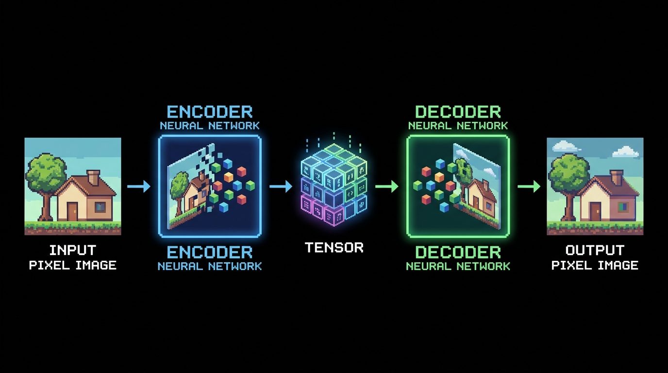
Essentially, the World Model architecture is made of three neural network modules:

• the Encoder answers the question “what is happening right now?”. It takes the input image and compresses it into a latent state (a tensor).

• the Dynamics answers the question “what happens next if I take this action?”. It’s the heart of the model, that takes the latent state (output of the Encoder) as input, and based on the action selected, predicts how the world changes (creates a simulated latent state).

• the Decoder shows what that predicted state looks like. It learns how to translate the compressed latent state back into something human-visible, like pixels.

import torch.nn as nnLATENT_SIZE = 128class Encoder(nn.Module):    def __init__(self):        super().__init__()        self.conv = nn.Sequential(            nn.Conv2d(1, 32,  kernel_size=4, stride=2, padding=1), nn.ReLU(),            nn.Conv2d(32,64,  kernel_size=4, stride=2, padding=1), nn.ReLU(),            nn.Conv2d(64,128, kernel_size=4, stride=2, padding=1), nn.ReLU(),            nn.Conv2d(128,128,kernel_size=4, stride=2, padding=1), nn.ReLU(),        )        self.fc = nn.Linear(128*4*4, LATENT_SIZE,)    def forward(self, x):        x = self.conv(x)        x = x.flatten(1)        return self.fc(x)class Decoder(nn.Module):    def __init__(self):        super().__init__()        self.fc = nn.Linear(LATENT_SIZE, 128*4*4,)        self.net = nn.Sequential(            nn.ConvTranspose2d(128,128,kernel_size=4, stride=2, padding=1), nn.ReLU(),            nn.ConvTranspose2d(128, 64,kernel_size=4, stride=2, padding=1), nn.ReLU(),            nn.ConvTranspose2d(64, 32, kernel_size=4, stride=2, padding=1), nn.ReLU(),            nn.ConvTranspose2d(32, 1,  kernel_size=4, stride=2, padding=1), nn.Sigmoid(),        )    def forward(self, z):        x = self.fc(z)        x = x.view(-1,128,4,4)        return self.net(x)

Please note that, at the moment, we just have the Encoder and Decoder (so-called Autoencoder architecture). If we pass a pixel image to the encoder, it would compress it into a latent state, and then if we give the output directly to the decoder (without going through the Dynamics), we’d get back almost exactly the same image. Why “almost”? During the Encoder compression, some information (e.g. some pixels) get inevitably lost, so the output of the Decoder will never be pixel-perfect.

The Dynamics module is used between the Encoder and the Decoder. The latent state (output of the Encoder) is passed to the Dynamics Neural Network, which predicts the next latent state. The important subtlety is that it isn’t predicting the pixel image directly, just the compressed version of it (the latent state), which is much easier.

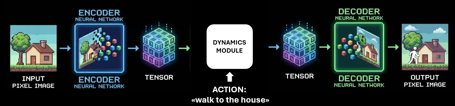
Basically, the Dynamics Neural Network must learn the game’s transition rules: “if the tank is here and I press LEFT, the next state should look like this; if I press FIRE, a projectile should appear; if an enemy is approaching, its position should change“.

class Dynamics(nn.Module):    def __init__(self):        super().__init__()        self.action_embedding = nn.Embedding(N_ACTIONS,32,)        self.net = nn.Sequential(            nn.Linear(LATENT_SIZE+32,256,), nn.ReLU(),            nn.Linear(256,256,), nn.ReLU(),            nn.Linear(256, LATENT_SIZE,),       )    def forward(self, latent, action,):        action = self.action_embedding(action)        x = torch.cat([latent,action,], dim=1,)        return self.net(x)

It’s time to train our World Model with the data stored into the Buffer (current image, action, next image). During the training, at each step, we will grab a batch of buffered experiences, the Encoder will compress them, the Dynamics tries to predict what the next compressed state should be, and the result is compared to the real observation to calculate the error (latent loss). At the same time, the Decoder turns the predicted latent into a pixel image, which is compared with the real next image (image loss). The model is optimized for the total loss (latent + image).

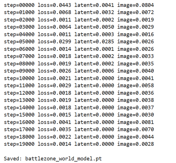
DEVICE = "cuda" if torch.cuda.is_available() else "cpu"LR = 1e-3TRAIN_STEPS = 20_000BATCH_SIZE = 64# WORLD MODELencoder = Encoder().to(DEVICE)dynamics = Dynamics().to(DEVICE)decoder = Decoder().to(DEVICE)optimizer = torch.optim.Adam(    list(encoder.parameters())    + list(dynamics.parameters())    + list(decoder.parameters()),    lr=LR,)# TRAINfor step in range(TRAIN_STEPS):    obs, actions, next_obs = buffer.sample(BATCH_SIZE)    obs = obs.to(DEVICE)    actions = actions.to(DEVICE)    next_obs = next_obs.to(DEVICE)        ##States    z = encoder(obs) #Current latent state    predicted_z = dynamics(z,actions) #Predict future latent state    with torch.no_grad():        target_z = encoder(next_obs) #Real future latent state    latent_loss = F.mse_loss(predicted_z, target_z) #Prediction loss        ##Obs    predicted_next_obs = decoder(predicted_z) #Reconstruct predicted future    image_loss = F.mse_loss(predicted_next_obs, next_obs) #Pixel reconstruction loss    ##Loss = state loss + obs loss    loss = (latent_loss + 0.5*image_loss)    optimizer.zero_grad()    loss.backward()    optimizer.step()    if step % 1_000 == 0:        print(            f"step={step:05d} "            f"loss={loss.item():.4f} "            f"latent={latent_loss.item():.4f} "            f"image={image_loss.item():.4f}"        )# SAVEtorch.save({    "encoder":encoder.state_dict(),    "dynamics": dynamics.state_dict(),    "decoder": decoder.state_dict(),    }, "battlezone_world_model.pt")print("nSaved: battlezone_world_model.pt")

Now, how do we test this? You have to show the model the current game screen, tell it you are taking an action, and ask “What should the next screen look like?”. First, I shall compress the current image into a latent state with the Encoder, pick a random action, and predict the next latent state with Dynamics. Then, I will transform the predicted latent state into a predicted pixel image with the Decoder.

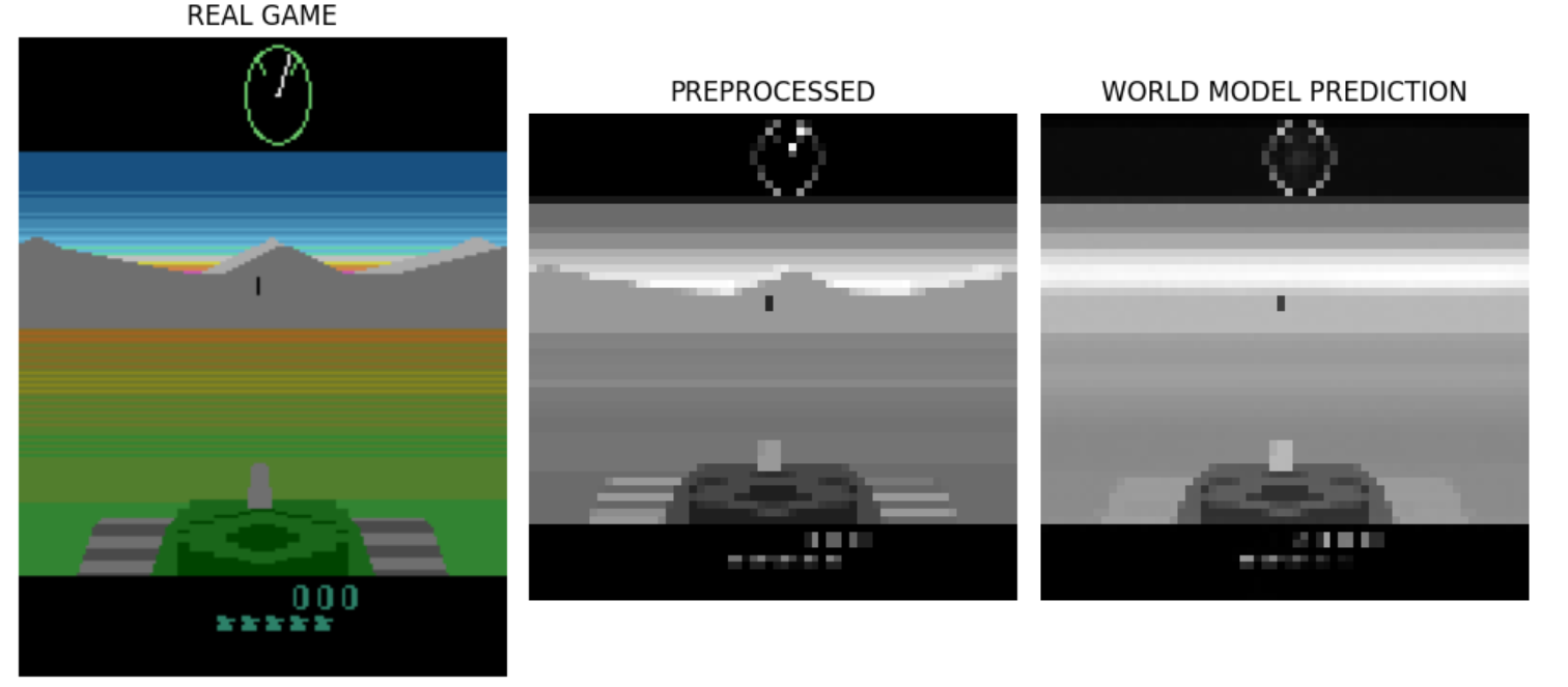
# LOADcheckpoint = torch.load("battlezone_world_model.pt", map_location=DEVICE)encoder = Encoder().to(DEVICE)dynamics = Dynamics().to(DEVICE)decoder = Decoder().to(DEVICE)encoder.load_state_dict(checkpoint["encoder"])dynamics.load_state_dict(checkpoint["dynamics"])decoder.load_state_dict(checkpoint["decoder"])encoder.eval()dynamics.eval()decoder.eval()# REAL OBSERVATIONobs, _ = env.reset()real_frame = preprocess(obs)frame = real_frame.unsqueeze(0).to(DEVICE) #add batch dimensionwith torch.no_grad():    z = encoder(frame)action = env.action_space.sample() #random actionprint("Testing action:", action)real_next_obs, reward, terminated, truncated, _ = env.step(action)real_next_frame = preprocess(real_next_obs).unsqueeze(0).to(DEVICE)# MODEL PREDICTIONwith torch.no_grad():    predicted_z = dynamics(z, torch.tensor([action], device=DEVICE))    predicted_frame = decoder(predicted_z)# VISUAL COMPARISONfig, axes = plt.subplots(1, 3, figsize=(10,5))axes[0].imshow(real_next_obs)axes[0].set_title("REAL GAME")axes[0].axis("off")axes[1].imshow(real_next_frame[0,0].cpu(), cmap="gray")axes[1].set_title("PREPROCESSED")axes[1].axis("off")axes[2].imshow(predicted_frame[0,0].cpu(), cmap="gray")axes[2].set_title("WORLD MODEL PREDICTION")axes[2].axis("off")plt.tight_layout()plt.show()

Please note that our dataset is made of grayscale low-resolution images, so the predictions look like that as well.

Full code on GitHub.

👉 Let’s Connect 👈