

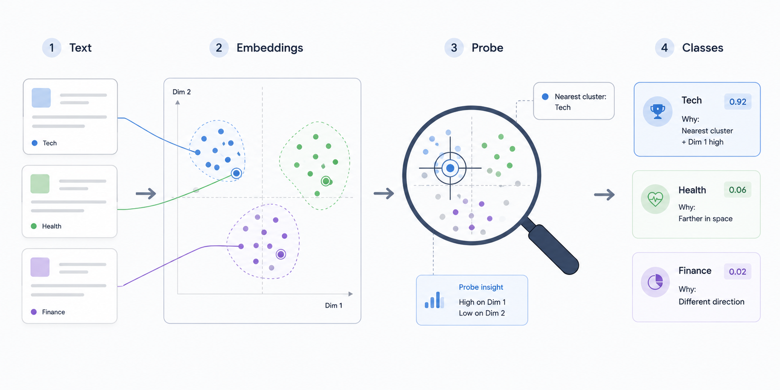
In this article, you will learn how to use probing classifiers, UMAP visualization, and SHAP values to interpret and analyze the quality of text embeddings generated by large language models.
Topics we will cover include:
- How to generate text embeddings from movie reviews using Scikit-LLM and a local Ollama model, and train a probing logistic regression classifier to evaluate their quality.
- How to use UMAP dimensionality reduction to visually inspect the semantic structure captured by LLM-generated embeddings.
- How to apply SHAP values to identify which latent embedding dimensions have the greatest influence on a classifier’s predictions.
Introduction
Text classification tasks have long been exclusively the domain of machine learning models and their direct “evolved form”: deep neural networks. However, we can’t deny that large language models (LLMs) have revolutionized the way text classifiers are now built, being more powerful and accurate but raising a side concern: the lack of interpretability due to LLMs being black-box models. Accordingly, when using an LLM before the core text classification task to convert raw text into embeddings — dense numerical vector representations of text — it is possible to capture semantic information. Yet one challenging question arises: what exactly is the model learning about text, and how does this internal learning process drive predictions?
This hands-on article shows how to use Scikit-LLM to generate embeddings, train a probing classifier, and unveil the black box by leveraging UMAP visualization and SHAP (SHapley Additive exPlanations) values: two popular explainable AI techniques for explaining model inference and decisions.
Initial Setup
The provided code here is fully compatible with Google Colab notebooks and requires installing the latest Scikit-LLM version. To keep the whole process cost-free, the code below shows how to configure everything for local, free execution. Let’s start by installing the following dependencies and packages, including the Ollama distributions for running local LLMs for free:
|
# 1. Installing Python libraries !pip install –q scikit–llm umap–learn shap
# 2. Fix Colab’s missing system dependencies first (version-dependent, use with care in other environments) !apt–get update –qq && apt–get install –y –qq zstd
# 3. Installing Ollama safely (thanks to zstd installed earlier) !curl –fsSL https://ollama.com/install.sh | sh
# 4. Starting the local server in the background and waiting for it to boot !nohup ollama serve > ollama.log 2>&1 & !sleep 5
# 5. Pulling the free embedding model: all-minilm !ollama pull all–minilm |
Now let’s import everything we will need:
|
import numpy as np import pandas as pd import matplotlib.pyplot as plt import umap import shap from skllm.config import SKLLMConfig from skllm.models.gpt.vectorization import GPTVectorizer from sklearn.model_selection import train_test_split from sklearn.linear_model import LogisticRegression from sklearn.metrics import classification_report from datasets import load_dataset |
Probing Embedding Spaces
The first step to probe and analyze Scikit-LLM embeddings is, of course, to get a fresh collection of them from a text dataset. We will first configure Scikit-LLM to point to a local Ollama server via "http://localhost:11434/v1/".
|
# 1. Pointing Scikit-LLM to the local Ollama server running in the background SKLLMConfig.set_gpt_url(“http://localhost:11434/v1/”) SKLLMConfig.set_openai_key(“dummy_key”) # Required format, but ignored locally |
After that, we use the public IMDB dataset containing movie reviews and load 1,000 of them: 500 labeled as positive and 500 labeled as negative, giving us a perfectly class-balanced sample. We use stratified sampling to keep 80% of the examples for training and the remaining 20% for testing:
|
1 2 3 4 5 6 7 8 9 10 11 12 13 14 15 16 17 |
# 2. Load one thousand movie reviews from IMDB dataset print(“Downloading and preparing IMDB dataset…”) dataset = load_dataset(“stanfordnlp/imdb”, split=“train”) df = dataset.to_pandas()
# Extracting 500 positive and 500 negative reviews to ensure a perfect balance df_pos = df[df[‘label’] == 1].sample(500, random_state=42) df_neg = df[df[‘label’] == 0].sample(500, random_state=42) df_balanced = pd.concat([df_pos, df_neg]).sample(frac=1, random_state=42) # Shuffle
texts = df_balanced[‘text’].tolist() labels = df_balanced[‘label’].values
# Splitting via stratified sampling X_train, X_test, y_train, y_test = train_test_split( texts, labels, test_size=0.2, random_state=42, stratify=labels ) |
We are now ready for the heaviest part of the process: generating embeddings for these 1,000 texts. We do so using Ollama’s all-minilm model via Scikit-LLM’s class designed for handling embedding models: GPTVectorizer. The syntax is intentionally similar to standard scikit-learn data transformations, as we can see:
|
# 3. Generating Embeddings using Scikit-LLM print(“Generating Embeddings…”) vectorizer = GPTVectorizer(model=“all-minilm”) X_train_vec = vectorizer.fit_transform(X_train) X_test_vec = vectorizer.transform(X_test) |
Be patient; if you are running this on Colab, it may take about 5–10 minutes to complete, as we are making 1,000 calls to a local LLM for embedding generation.
A probing classifier (or a probing model) is a diagnostic tool used to inspect the internal representations built by complex models. How can we reliably determine that the embeddings generated earlier have enough quality to separate the data into classes — positive vs. negative reviews — properly? One way is to use a smaller, simpler classifier, such as logistic regression, and examine the accuracy metrics. If a classification report — described by precision, recall, and F1 scores per class — yields decent results even for this shallow classifier, that indicates the embeddings are rich enough for the classification task. Using a simpler classifier as our probing model also helps isolate the contribution being attributed to the embeddings themselves.
|
# 4. Training the Probing Classifier print(“nTraining Classifier…”) clf = LogisticRegression(random_state=42, max_iter=1000) clf.fit(X_train_vec, y_train) print(classification_report(y_test, clf.predict(X_test_vec))) |
Results:
|
Training Classifier... precision recall f1–score support
0 0.77 0.76 0.76 100 1 0.76 0.77 0.77 100
accuracy 0.77 200 macro avg 0.77 0.77 0.76 200 weighted avg 0.77 0.77 0.76 200 |
Considering that the dataset size is not extraordinarily large relative to the embedding dimensionality, these results are quite respectable for a simple, linear classifier like logistic regression, which is typically applied to smaller, purely tabular datasets.
Let’s look at another introspection tool: UMAP (Uniform Manifold Approximation and Projection). UMAP is a projection-based dimensionality reduction technique commonly used for visualization. We project the embeddings down to 2 dimensions using cosine similarity as the distance metric, which is standard when working with text embeddings. The resulting scatterplot helps us determine whether there is any natural grouping between embeddings associated with positive and negative reviews:
|
1 2 3 4 5 6 7 8 9 10 11 12 13 14 15 16 17 18 19 20 21 22 23 |
# 5. Visualize with UMAP print(“Running UMAP Projection…”) reducer = umap.UMAP( n_components=2, metric=‘cosine’, # Native metric for transformer embeddings n_neighbors=30, # Captures broader global structure min_dist=0.1, # Prevents excessive point overlap random_state=42 ) X_umap = reducer.fit_transform(X_train_vec)
plt.figure(figsize=(9, 6)) scatter = plt.scatter( X_umap[:, 0], X_umap[:, 1], c=y_train, cmap=‘coolwarm’, s=25, # Smaller marker size alpha=0.6, # Transparency reveals true density edgecolors=‘none’ # Eliminates border clutter ) plt.title(“UMAP Projection of Scikit-LLM Embeddings”) plt.show() |
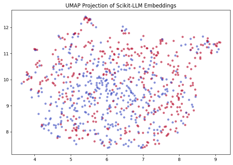
The results are not extraordinary at first glance — there is no near-perfect class-wise separation between reviews — but considering these are LLM-generated embeddings heavily projected into just two dimensions, a subtle sense of grouping is still visible: the southern half of the plot shows a dominance of negative reviews (blue dots), while the upper half has a majority of positive reviews (fuchsia).
Last, we can resort to one of the most popular frameworks for examining machine learning model behavior: SHAP (SHapley Additive exPlanations). SHAP can help us understand which of the latent dimensions (features) in our embeddings had the most influence on the probing classifier’s predictions.
The code below constructs a SHAP summary plot that visualizes which embedding dimensions exert the most impact on model classifications. By default, the plot displays the top 20 features with the largest overall impact, using color to indicate whether each feature contributes toward positive or negative classifications depending on whether its values are higher or lower.
|
1 2 3 4 5 6 7 8 9 10 11 12 13 14 15 16 17 18 |
# 6. Extracting Feature Importance with SHAP print(“Calculating SHAP values…”) explainer = shap.LinearExplainer(clf, X_train_vec) shap_values = explainer.shap_values(X_test_vec)
# Standardizing SHAP output format across different scikit-learn versions if isinstance(shap_values, list): shap_values = shap_values[1]
plt.figure(figsize=(8, 5)) shap.summary_plot( shap_values, X_test_vec, feature_names=[f“Dim {i}” for i in range(X_train_vec.shape[1])], show=False ) plt.title(“SHAP Summary: Most Impactful Latent Dimensions”) plt.show() |
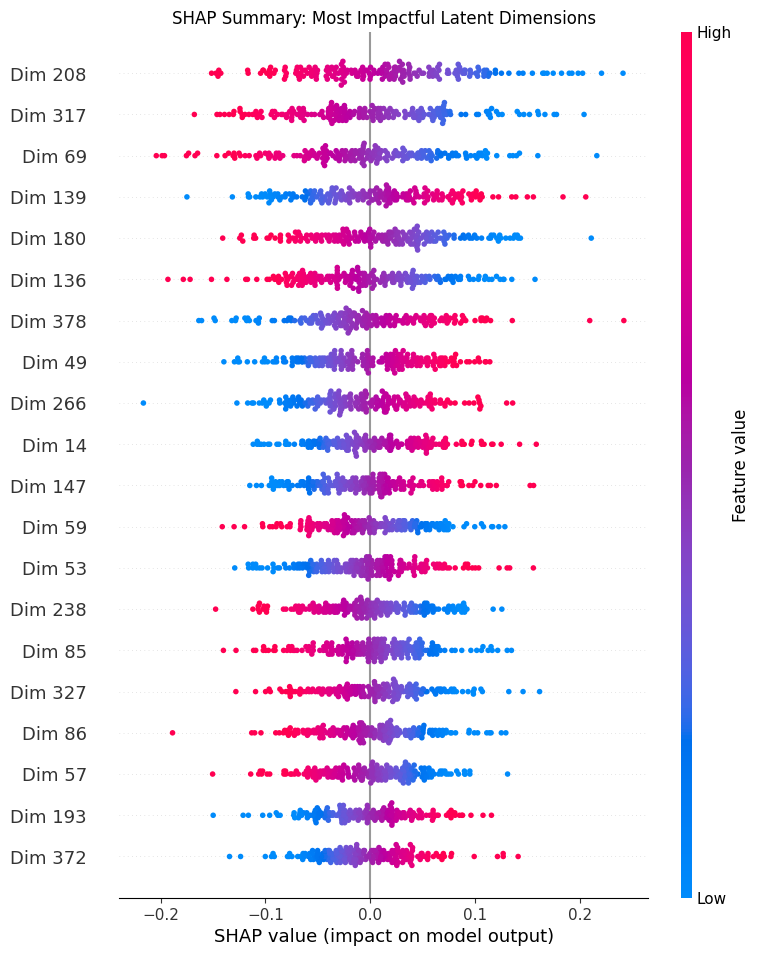
We can conclude that dimension 208 is the primary signal for negative reviews, closely followed by dimension 317. Meanwhile, dimension 139 is the main driver for positive reviews, as higher values (pink) for this feature push the model’s raw prediction toward higher values (the right-hand side of the plot, leaning toward the positive class).
Conclusion
This article illustrated how to use a probing classification model, along with visualization tools like UMAP and SHAP, to better understand and interpret the nature and quality of text embeddings produced by LLMs for downstream machine learning tasks like text classification. We relied on Scikit-LLM, a library that mirrors scikit-learn’s API to seamlessly integrate LLMs into a variety of tasks, including embedding generation from raw text such as movie reviews.