Seizing the Moment: The Hidden Silhouette of Data

Section 0: Abstract

If you’ve spent any time in statistics or machine learning, you’ve met the usual suspects: the mean and the variance. If you’re feeling brave, you might even look at skewness or kurtosis. In day-to-day data analysis, it is easy to treat these metrics as a disjointed collection of individual tools — a patchwork utility belt of sorts.

You’ve probably heard of statistical moments, or, if, unlike me, you have a background in physics, you may find terms like torque (the moment of force) or the moment of inertia (the second moment of mass) familiar.

Regardless of your field, the underlying systems overlap, largely because of cross-pollination between the two fields.

The Premise

The main point of this article is answering the question of what value moments add if we already have the tools necessary to talk about distributions — the mean, the variance, skewness, and kurtosis. Secondly, I discuss some analytical and theoretical applications of moments, focusing on machine learning and statistics.

To start, I’ll lay out some concrete definitions before we get into the slightly more opinionated parts of this article.

···

Section 1: How do we define moments in statistics?

In statistics, a moment is simply the quantitative measure of the shape of a set of points or a probability distribution. Mathematically, they come in two main flavors: raw moments (taken around zero) and central moments (taken around the mean).

If we have a random variable, the $n-$th raw moment is defined as the expected value of$X$raised to the power of$n$:

When $n=1$

To look at the features of a shape independently of where it is located on a graph, we shift the variable by subtracting the mean. This gives us the$n$-th central moment:

The 1st Central Moment is always 0, because$E[X – mu] = mu – mu = 0$

The 2nd Central Moment is the variance $(sigma^2)$, measuring the dispersion around the center.

To go higher, we need to strip away the distorting effects of scale. We do this by dividing by the standard deviation ($sigma$) raised to that same power, giving us standardized moments:

The 3rd Standardized Moment is skewness, quantifying directional asymmetry.

The 4th Standardized Moment is kurtosis, capturing tail weight and peak sharpness.

Notice how computing the first two standardized moments would be trivial because every distribution is centered or variance-standardized with respect to itself.

For the 1st Standardized Moment for any distribution:

And for the 2nd Standardized Moment for any distribution:

···

Section 2: What’s the point of moments?

This brings us to the core premise: If we already have the mean, variance, skewness, and kurtosis, why do we need to encapsulate them under an abstract umbrella called “moments”? What value does this addition bring?

The short answer is that moments are not a competing framework. You aren’t overcomplicating your math by learning them, because you are already using them. “Moments” is simply the formal, unified family name for the exact measurements you know.

To see why this grouping matters, consider an algebraic parallel. Imagine a scenario where we treated a squared number $x^2$, a cubed number $x^3$, and a biquadratic number $x^4$ as completely unrelated, independent operations. Without a unifying theory, each would require isolated textbook chapters, distinct nomenclature, and separate rules.

The explicit concept of an exponent $x^n$dissolves that artificial separation between squares, cubes and so on.

You instantly realize that squares and cubes aren’t disparate ideas; they are just different iterations of the exact same underlying engine. Setting $n=2$

Statistical moments serve the exact same structural purpose for data distributions. The mean, variance, skewness, and kurtosis are not isolated metrics. They are simply expectations of the 1st, 2nd, 3rd, and 4th powers of a random variable, bound together by a single mathematical law.

Grouping them this way changes how we handle data. Instead of writing separate algorithms or proofs to handle variance or skewness, we can construct generalized mathematical tools that manipulate the $n$-th power of a distribution directly.

···

Section 3: The Moment Generating Function (MGF)

Once we accept that mean, variance, skewness, and kurtosis are just low-order exponents of a distribution, the next logical step is to find a way to manage all of them simultaneously. We don’t want to stop at the 4th power. We want a unified mathematical machine that can hold the entire infinite chain of a distribution’s powers.

That machine is the Moment Generating Function (MGF).

For a random variable$X$, the MGF is defined as the expected value of $e^{tX}$:

Introducing the constant $e$ might look like an arbitrary complication, but this choice is entirely intentional, and driven by calculus. The Taylor series expansion for $e^z$ is built completely out of increasing powers:

If we substitute $z = tX$

Because expectation is a linear operator, taking the expected value$E[cdot]$ allows us to pass the expectation inside the summation, applying it directly to the random variables:

Look closely at what just happened. The MGF is not a single value; it is a mathematical clothesline, and the raw moments are the clothes pinned to it. The first moment $E[X]$ is pinned to $t$ the second moment$E[X^2]$ is pinned to $t^2$ and the $n$-th moment is pinned to $t^n$.

To empirically prove that this clothesline works, you can run a simple simulation. If we take a standard Exponential distribution with $lambda = 1$

The case for t

To understand what the parameter t actually means, think of it as a continuous spatial warp.

When you evaluate the MGF, you are multiplying your data’s original distribution’s silhouette by an exponential ramp, $e^{tX}$. The variable t is simply the volume dial for that ramp.

Imagine a perfectly flat Uniform distribution from 0 to 10—a flat brick of data.

• At t = 0: The exponential ramp $e^{0 cdot X}$ is a perfectly flat line at 1. Multiplying your brick by 1 changes nothing. The total area under the curve is just 1 (the total probability).

• At t = 0.1: You apply a mild exponential slope. The value at $X=0$

• At t = 0.2: You double the dial. The ramp climbs steeply. The value at$X=10$

By continuously turning the dial of t away from zero, you create a smooth, continuous tracking curve,$M_X(t)$

The MGF Uniqueness Theorem: If two distributions share the exact same MGF in a local neighborhood around zero, they share the exact same infinite sequence of moments. And if they share the exact same infinite sequence of moments, they are guaranteed to be the exact same distribution.

But why is it impossible for two completely different distribution silhouettes to generate the exact same converging MGF curve?

The rigidity is enforced by a core property of power series: A convergent Taylor series defines an analytic function, and analytic functions are completely locked in space.

If you have an infinite list of moments, you can build a Taylor series out of them. If that series converges to a finite value across an open interval of t around zero, it creates a single, smooth, continuous curve. In mathematics, two different analytic curves cannot intersect along a continuous line and then split apart later. If they match perfectly along a continuous segment of t, they are locked into matching perfectly everywhere.

Because there is a flawless, rigid 1-to-1 mechanical bond between the continuous shape of the $M_X(t)$

By scaling up the exponent analogy into an infinite polynomial, the MGF allows you to package a distribution’s entire structural identity into a single, derivable function.

···

Section 4: Moments when moments don’t work

Up to this point, our mathematical narrative feels airtight: moments act as exponents of shape, the MGF collects an infinite sequence of these traits, and the Uniqueness Theorem guarantees that this sequence maps to one—and only one—distribution. It implies a comforting law: if you know every single moment from now until infinity, you uniquely define the exact shape of your data.

But there is a massive catch. In advanced probability theory, this is known as the Hamburger Moment Problem which unfortunately has nothing to do with hamburgers and was named after Hans Ludwig Hamburger. It introduces a fascinating blind spot into data analysis.

The Uniqueness Theorem only holds true if the moments don’t grow too fast. If a distribution has incredibly thick, heavy tails, the MGF fails to converge, and the entire framework fractures. The classic, mind-bending exception to the rule is the Log-Normal distribution.

Imagine a standard log-normal probability density function, which we can call $f_{0}(x)$

Where (a) is a perturbation constant between 0 and 1. Visually, these two distributions look completely different. One is a smooth, predictable asymmetric curve; the other has a distinct, periodic ripple embedded along its heavy tail. They represent two completely unique silhouettes.

Yet, if you calculate the 1st moment, the 2nd moment, the 3rd moment, or even the 1,000,000th raw moment of both distributions via integration, they match identically down to the last decimal place.

A simple script to validate this collapse:

import mathimport numpy as npimport scipy.integrate as integrateimport plotly.graph_objects as gofrom plotly.subplots import make_subplots# -------------------------------------------------------------------------# 1. DISTRIBUTION DEFINITIONS# -------------------------------------------------------------------------def f_0(x):    """Standard Log-Normal PDF with safe vectorized support handling."""    x_arr = np.asarray(x, dtype=float)    pdf = np.zeros_like(x_arr)    pos = x_arr > 0    pdf[pos] = (1.0 / (x_arr[pos] * np.sqrt(2.0 * np.pi))) * np.exp(- (np.log(x_arr[pos])**2) / 2.0)    return pdf if pdf.ndim > 0 else pdf.item()def f_a(x, a=0.5):    """Wavy Log-Normal Twin (Identical moments, distinct silhouette)."""    x_arr = np.asarray(x, dtype=float)    return f_0(x_arr) * (1.0 + a * np.sin(2.0 * np.pi * np.log(np.where(x_arr > 0, x_arr, 1.0))))# -------------------------------------------------------------------------# 2. COMPUTE FINITE MOMENTS AND ACCUMULATE PARTIAL MGF SUMS# -------------------------------------------------------------------------orders = np.arange(1, 11)moments_base = []moments_twin = []t = 0.05  # Small scaling variable for MGF evaluationmgf_sums_base = [1.0]mgf_sums_twin = [1.0]for n in orders:    m_base = float(np.exp((n**2) / 2.0))        # Integrating in z-space: z = ln(x) - n    # The integrand is strictly odd, yielding ~0 without roundoff blowup    perturbation, _ = integrate.quad(        lambda z: np.exp(-0.5 * z**2) * np.sin(2.0 * np.pi * z),        -8, 8    )    perturbation *= (0.5 * m_base / np.sqrt(2.0 * np.pi))    m_twin = m_base + perturbation        moments_base.append(m_base)    moments_twin.append(m_twin)        term_base = (t**n / math.factorial(n)) * m_base    term_twin = (t**n / math.factorial(n)) * m_twin        mgf_sums_base.append(mgf_sums_base[-1] + term_base)    mgf_sums_twin.append(mgf_sums_twin[-1] + term_twin)# -------------------------------------------------------------------------# 3. INTERACTIVE PLOTLY VISUALIZATION (2x2 GRID)# -------------------------------------------------------------------------fig = make_subplots(    rows=2, cols=2,     subplot_titles=(        "Standard Log-Normal Density Function f_0(x)",         "Wavy Twin Density Function f_a(x)",        "Moment Parity Plot (Log-Log Scale)",         "MGF Taylor Series Partial Sum Explosion"    ))x_grid = np.linspace(0.01, 5.0, 500)y_base_pdf = f_0(x_grid)y_twin_pdf = f_a(x_grid)# --- Top Row: Probability Density Functions ---fig.add_trace(go.Scatter(    x=x_grid, y=y_base_pdf,    mode='lines', line=dict(color='blue', width=2),    name='Base Log-Normal'), row=1, col=1)fig.add_trace(go.Scatter(    x=x_grid, y=y_twin_pdf,    mode='lines', line=dict(color='red', width=2, dash='dash'),    name='Wavy Twin (a=0.5)'), row=1, col=2)# --- Bottom Left: Direct Moment Comparison ---fig.add_trace(go.Scatter(    x=moments_base, y=moments_twin,    mode='markers+lines',    marker=dict(color='purple', size=8),    line=dict(color='purple', width=1.5),    name='Moment Value Matches'), row=2, col=1)min_val, max_val = min(moments_base), max(moments_base)fig.add_trace(go.Scatter(    x=[min_val, max_val], y=[min_val, max_val],    mode='lines', line=dict(color='black', dash='dash', width=1),    name='Perfect Identity (Y = X)'), row=2, col=1)# --- Bottom Right: MGF Partial Sum Divergence ---iterations = np.arange(0, len(mgf_sums_base))fig.add_trace(go.Scatter(    x=iterations, y=mgf_sums_base,    mode='lines+markers', line=dict(color='blue', width=2),    name='Base MGF Sum'), row=2, col=2)fig.add_trace(go.Scatter(    x=iterations, y=mgf_sums_twin,    mode='lines+markers', line=dict(color='red', width=2, dash='dash'),    name='Wavy Twin MGF Sum'), row=2, col=2)fig.update_layout(    title_text="The Failure of Convergence: Unveiling the Hamburger Moment Problem",    template="plotly_white",    width=1100, height=900,    hovermode="x unified")fig.update_xaxes(title_text="x", row=1, col=1)fig.update_yaxes(title_text="Probability Density", row=1, col=1)fig.update_xaxes(title_text="x", row=1, col=2)fig.update_yaxes(title_text="Probability Density", row=1, col=2)fig.update_xaxes(title_text="Base Log-Normal Moments", type="log", row=2, col=1)fig.update_yaxes(title_text="Wavy Twin Moments", type="log", row=2, col=1)fig.update_xaxes(title_text="Number of Moments Added to Sum", row=2, col=2)fig.update_yaxes(title_text="Calculated MGF Value", type="log", row=2, col=2)fig.show()

The plot shows us how moments sometimes don’t do what they’re supposed to. The top two subplots show the actual pdfs of the standard log normal and a modified one. The bottom two explain that the diverging moments make the moment equivalency invalid.

Two completely different curves yet they have the same moments.

This empirical reality delivers a critical lesson for statistical modeling. Moments only hold the complete structural identity of your data if the distribution satisfies Carleman’s Condition—a rule stating that the sum of the reciprocal roots of the moments must diverge. When data has extreme tail behavior, the infinite chain of exponents leaks information, proving that moments are a powerful summary framework, but not an absolute guarantee of identity.

Note:

Because the log-normal distribution is restricted to the non-negative half-line, this is technically a manifestation of the Stieltjes moment problem, the half-line cousin of Hamburger’s theorem—both demonstrating the failure of moment determinacy. But the underlying principle is exactly the same.

···

Section 5: Applications

Once you peel back the abstraction, you realize that higher-order exponents are not just theoretical constructs for proofs. They form the explicit infrastructure of the machine learning algorithms we use every day. When an optimizer or an evaluation metric needs to understand the shape of loss landscapes, gradients, or feature distributions, it deploys statistical moments. Here are some common applications of moments:

1. Neural Network Optimization

The Adam Optimizer The most widely used training algorithm in deep learning, Adam, literally stands for Adaptive Moment Estimation. When a model calculates gradients during backpropagation, the values oscillate wildly across the loss landscape. To stabilize training, Adam tracks two distinct running metrics across every single parameter weight:

The 1st Moment (Mean): Adam computes an exponentially decaying moving average of the gradient, denoted as $m_t$

The 2nd Uncentered Moment (Variance-adjacent): It simultaneously tracks a moving average of the squared gradients, denoted as $v_t$

By dividing the mean gradient by its variance signature, Adam dynamically scales the learning rate for every single parameter. If a weight’s gradients are highly volatile (high variance), Adam scales down the step size. If a weight’s gradients are steady and consistent (low variance), Adam accelerates down the path. It is moment-driven engineering at a massive scale.

2. Evaluating Generative Models via Fréchet Inception Distance (FID)

When training a Generative Adversarial Network (GAN) or a Diffusion model to generate images, we cannot easily compute a traditional loss function like mean squared error. If a model generates a hyper-realistic image of a cat but shifts it two pixels to the right, a pixel-by-pixel error check will flag it as a complete failure.

To evaluate image quality accurately, we use the Fréchet Inception Distance (FID). FID works by feeding a batch of real images and a batch of generated images through a computer vision model Instead of looking at pixels, it extracts the raw activations from the final pooling layer, mapping the images into a high-dimensional feature space.

To evaluate if the generated images look authentic, FID checks if the silhouette of the generated features matches the silhouette of the real features. It does this by computing the two lowest-order moments of both feature spaces:

• The mean vector ($mu$, the 1st moment) to locate the center of the feature clusters.

• The covariance matrix ($Sigma$, the 2nd joint moment) to measure the spread and geometric orientation of the shapes. It then calculates the geometric distance between these two multi-dimensional silhouettes. If the generated images are clean, diverse, and realistic, their 1st and 2nd moments will align perfectly with the real data distribution, driving the FID score down toward zero.

3. Method of Moments

It is worth looking at how moments solve a classic statistical machine learning challenge: parameter estimation. When you have a raw data vector and assume it fits a specific distribution family, how do you back-calculate the hidden parameters that generated it?

This is where the Method of Moments (MoM) comes in.

Instead of setting up complex, iterative optimization loops, the Method of Moments uses a brute-force algebraic shortcut. It operates on a beautifully simple premise: If you want to estimate the hidden parameters of a population, calculate the sample moments from your data array and match them directly to the theoretical population moments.

This creates a clean system of equations where you force your empirical observations to match the theoretical shapes:

To understand what MoM actually is, it helps to contrast it directly with the industry standard: Maximum Likelihood Estimation (MLE). The divergence between these two approaches reveals a fundamental trade-off between structural centers of mass and strict probability boundaries.

The Intuition: Structural Mass vs. Boundary Probability

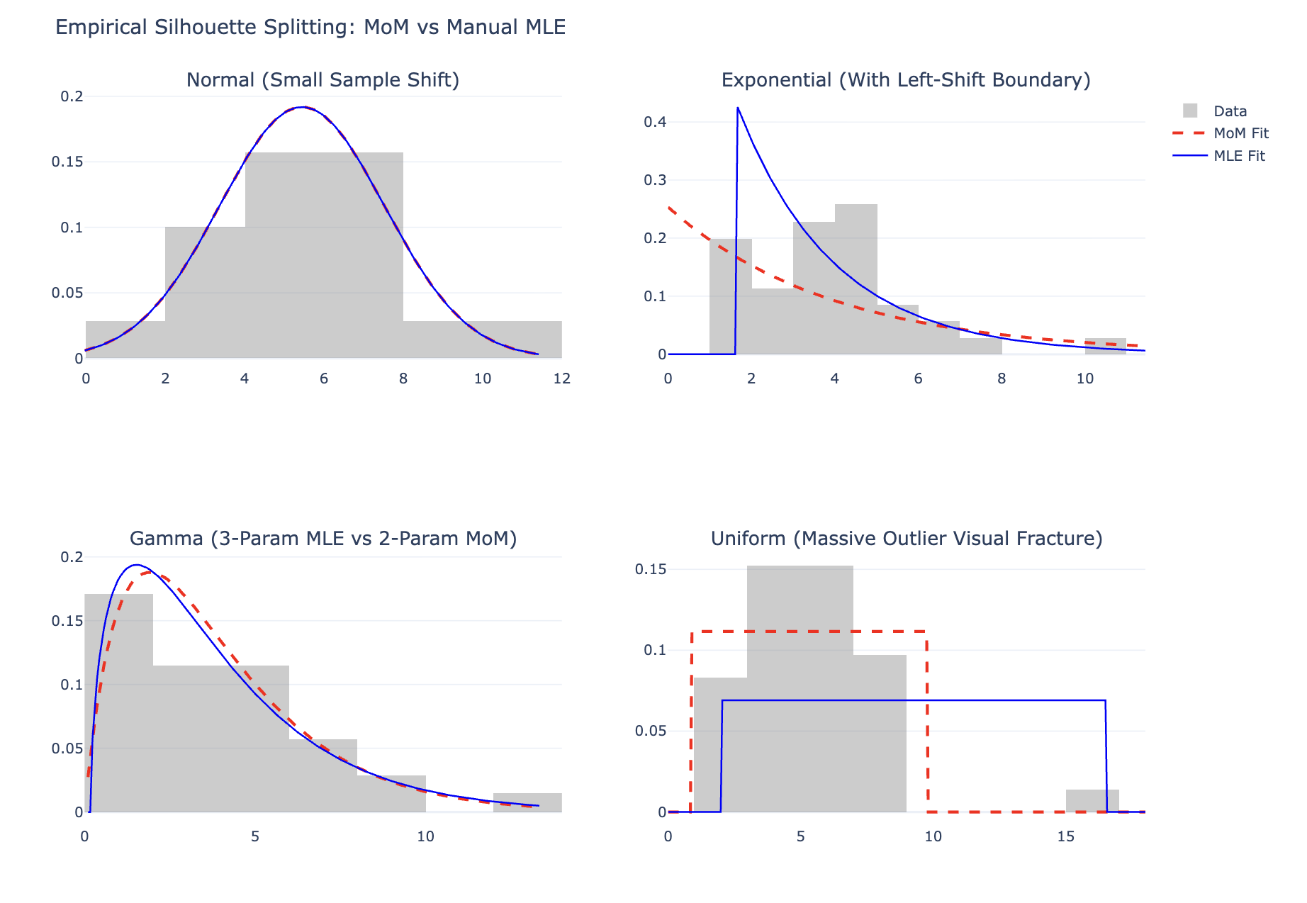
• MLE seeks to maximize joint probability. It asks: What parameters make observing this exact dataset as likely as possible? For distributions like the Uniform distribution continuous over $[a, b]$, the joint likelihood drops to exactly zero if even a single observed data point falls outside those walls. If you have a dataset spanning from 2 to 8, and append a massive artificial outlier at 16.5, the MLE boundary is forced to stretch all the way to 16.5 to avoid a total likelihood collapse. A single freak point completely dictates the model edge.

• MoM optimizes for structural mass. It treats data points like a collective physical system. Adding that outlier at 16.5 shifts the sample mean slightly to the right and increases the variance, but because these metrics are calculated as averages ($frac{1}{N} sum x_i$

The Computational Reality: Analytical Closed Forms vs. Numerical Loops

This brings up a massive engineering advantage for MoM. To find an MLE solution, you must take the derivative of the log-likelihood function, set it to zero, and solve.

Whether MLE has an analytical, closed-form solution depends entirely on the specific distribution family. For Normal distributions, the MLE matches your raw sample mean and variance. For Uniform distributions, it matches your sample minimum and maximum.

But for distributions like the Gamma distribution, the log-likelihood equation involves a non-algebraic digamma function. Because of this, MLE is completely impossible to solve with standard algebra. You are forced to write a numerical optimization loop (like minimizing the negative log-likelihood) to let a computer search for the peak iteratively.

The Method of Moments completely bypasses this computational tax. A Gamma distribution is governed by a shape parameter ($alpha$) and a scale parameter ($beta$). Analytically, its first two theoretical moments are neatly tied to these parameters:

• First Moment (Mean): $E[X] = alphabeta$

• Second Central Moment (Variance):$Var(X) = alphabeta^2$

By calculating your empirical sample mean ($bar{X}$

Even for the Gamma distribution, MoM gives you cheap, closed-form equations that evaluate instantly without a single gradient evaluation or optimization step.

You can visualize this exact divergence in parameter estimation behavior by executing the clean, modular Plotly script below. It abstracts the rendering logic into a single trace utility while keeping the manual mathematical calculations explicit for each distribution family.

import mathimport numpy as npimport plotly.graph_objects as gofrom plotly.subplots import make_subplotsfrom scipy.optimize import minimizefrom scipy.special import gamma as gamma_funcnp.random.seed(101)N = 35def add_subplot_traces(fig, row, col, data, x_grid, pdf_mom, pdf_mle):    is_first = (row == 1 and col == 1)    fig.add_trace(go.Histogram(        x=data, histnorm='probability density', marker_color='gray',         opacity=0.4, showlegend=is_first, name="Data"    ), row=row, col=col)    fig.add_trace(go.Scatter(        x=x_grid, y=pdf_mom, line=dict(color='red', width=2.5, dash='dash'),         showlegend=is_first, name="MoM Fit"    ), row=row, col=col)    fig.add_trace(go.Scatter(        x=x_grid, y=pdf_mle, line=dict(color='blue', width=1.5),         showlegend=is_first, name="MLE Fit"    ), row=row, col=col)# 1. GENERATE DATASETSdata_normal = np.random.normal(loc=5.0, scale=2.0, size=N)data_exponential = np.random.exponential(scale=3.0, size=N) + 1.5data_gamma = np.random.gamma(shape=2.0, scale=2.0, size=N)data_uniform = np.append(np.random.uniform(low=2.0, high=8.0, size=N), [16.5])fig = make_subplots(    rows=2, cols=2,     subplot_titles=(        "Normal (MLE & MoM Equivalence)",         "Exponential (Shifted Support Boundary)",         "Gamma (Numerical MLE vs Closed MoM)",         "Uniform (Outlier Leverage Split)"    ))# Subplot 1: Normald = data_normalx = np.linspace(min(d) - 1, max(d) + 1, 200)mu, sigma = np.mean(d), np.std(d)pdf_norm = (1.0 / (sigma * np.sqrt(2 * np.pi))) * np.exp(-0.5 * ((x - mu) / sigma) ** 2)add_subplot_traces(fig, 1, 1, d, x, pdf_norm, pdf_norm)# Subplot 2: Exponential (Shifted)d = data_exponentialx = np.linspace(0, max(d) + 1, 200)scale_mom = np.mean(d)loc_mle = np.min(d)scale_mle = np.mean(d) - loc_mlepdf_mom = np.where(x >= 0, (1.0 / scale_mom) * np.exp(-x / scale_mom), 0.0)pdf_mle = np.where(x >= loc_mle, (1.0 / scale_mle) * np.exp(-(x - loc_mle) / scale_mle), 0.0)add_subplot_traces(fig, 1, 2, d, x, pdf_mom, pdf_mle)# Subplot 3: Gamma (2-Param: alpha=shape, beta=scale)d = data_gammax = np.linspace(0.01, max(d) + 1, 200)mean_val, var_val = np.mean(d), np.var(d)alpha_mom = (mean_val ** 2) / var_valbeta_mom = var_val / mean_valdef gamma_nll(params):    a, b = params    if a <= 0 or b <= 0:        return 1e10    return -np.sum((a - 1) * np.log(d) - (d / b) - a * np.log(b) - math.lgamma(a))res = minimize(gamma_nll, [1.0, 1.0], method='Nelder-Mead')alpha_mle, beta_mle = res.xpdf_gamma_mom = (x**(alpha_mom - 1) * np.exp(-x / beta_mom)) / (beta_mom**alpha_mom * gamma_func(alpha_mom))pdf_gamma_mle = (x**(alpha_mle - 1) * np.exp(-x / beta_mle)) / (beta_mle**alpha_mle * gamma_func(alpha_mle))add_subplot_traces(fig, 2, 1, d, x, pdf_gamma_mom, pdf_gamma_mle)# Subplot 4: Uniform with Outlierd = data_uniformx = np.linspace(0, 18, 300)mean_u, var_u = np.mean(d), np.var(d)a_mom = mean_u - np.sqrt(3 * var_u)b_mom = mean_u + np.sqrt(3 * var_u)a_mle, b_mle = np.min(d), np.max(d)pdf_u_mom = np.where((x >= a_mom) & (x <= b_mom), 1.0 / (b_mom - a_mom), 0.0)pdf_u_mle = np.where((x >= a_mle) & (x <= b_mle), 1.0 / (b_mle - a_mle), 0.0)add_subplot_traces(fig, 2, 2, d, x, pdf_u_mom, pdf_u_mle)fig.update_layout(    title_text="Empirical Silhouette Splitting: MoM vs MLE",    template="plotly_white",    width=1100, height=800,    hovermode="x unified")fig.show()

While MLE remains structurally necessary for small, clean datasets due to its minimum possible variance properties, the Method of Moments functions as an essential, high-speed baseline estimator. It acts as a direct validation that treating your data features as a sequence of rising geometric powers allows you to resolve spatial distributions instantly with nothing but basic arithmetic.

···

Section 6: In Conclusion

Ultimately, statistical moments are not just an isolated checklist of descriptive tools; they form an infinite, additive coordinate engine that can pack a distribution’s entire structural identity into a single function.

By introducing the external parameter t, the Moment Generating Function acts as a continuous spatial scanner, leveraging the rigid calculus of a convergent power series to guarantee a unique 1-to-1 mapping back to a single distribution silhouette.

Whether you are scaling gradient step sizes in the Adam optimizer, computing feature distances with the FID score, or deploying the algebraic shortcuts of the Method of Moments, understanding moments means understanding the trade-offs of structural compression.

···

Section 7: References and Citations

1. The Uniqueness Criterion: Carleman’s Condition provides the foundational, rigorous mathematical checkpoint determining whether an infinite sequence of moments possesses the tight convergence bounds required to uniquely lock in a distribution’s identity on an open real interval. For the foundational proof showing how tight convergence bounds determine whether a sequence uniquely locks in a distribution’s identity, see the mathematical derivation of determinacy criteria in Ten Lectures on the Moment Problem (arXiv).

2. The Hamburger Moment Problem: The Hamburger Moment Problem establishes the definite proof that on an infinite domain, an under-determined system of integration constraints allows multiple unique probability density functions to yield the exact same sequence of moments simultaneously if the tails decay too slowly. For a detailed derivation, please look at this thesis by Ayoola Jinadu:

3. Moment Estimation Standards: Pearson, K. (1894). “Contributions to the Mathematical Theory of Evolution.” Philosophical Transactions of the Royal Society of London A. This foundational work introduced the Method of Moments, establishing the direct algebraic bridge used to estimate population parameters by explicitly matching empirical sample data traits to theoretical curves.

4. Deep Learning Implementations: Kingma, D. P., & Ba, J. (2014). “Adam: A Method for Stochastic Optimization.” International Conference on Learning Representations (ICLR). Section 2 outlines the algorithmic mechanics of modern neural network training, detailing how parameter trajectories are dynamically smoothed using moving averages of the first moment (mean gradient) and second uncentered moment (gradient variance signature).