

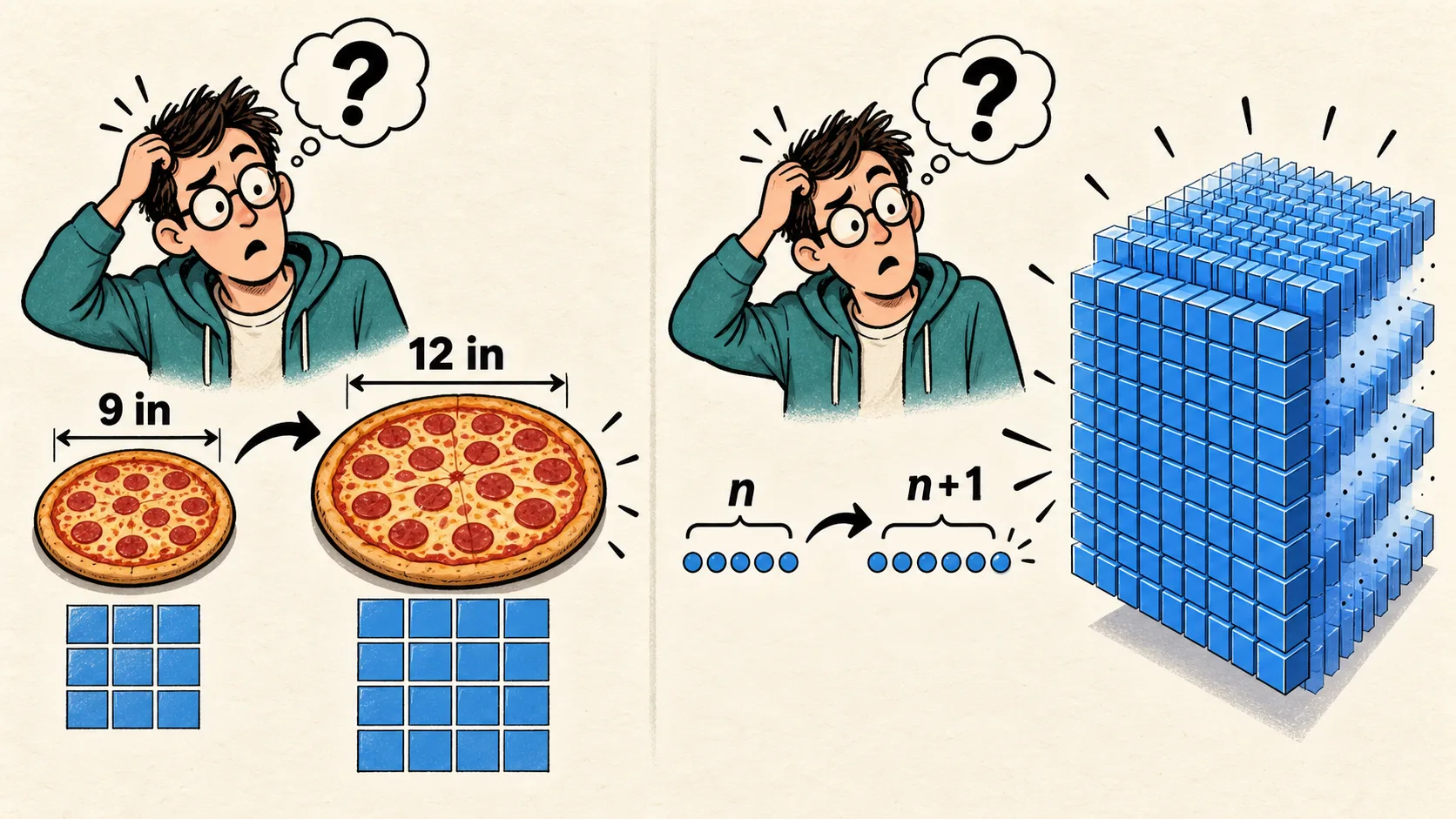
A 12-inch pizza is not half again as much pizza as an 8-inch one. It is 2.25x as much. This is because the pizza’s area follows the square of its radius. People generally have poor intuition for areas, or any thing that grows quicker than its linear boundaries. This is why pizzerias price by diameter and customers reliably buy pizzas they can’t finish.
The same failure of intuition sat inside a client’s 3D scan-matching pipeline for the best part of a year. It cost them double the memory on every worker in the fleet. Somewhere in the scoring code was a table with one row and one column per element. Everybody who read that code saw a list when they should have seen a square. This is an account of finding it, of the four ways a square like that can be bounded, and of why we chose the slowest.
The Problem
The pipeline aligns two surface scans, subtracts one from the other, and inspects what is left over. If the two scans are of the same object then the leftover is nothing. One class of scanner has a known failure mode: where the object has a flat face, the scanner sometimes records a shallow pyramid instead. Left in the data, those pyramids look like real geometric differences and cause a true match to be rejected. So before we mark two items as matching, we check whether the leftover shell is pyramid-shaped. If it is the pyramid pieces are removed from the objects, rather than being considered as evidence of a match.
Detecting a pyramid means finding its flat base, and the scorer finds the base by looking at surface orientation. Every triangle on the mesh has a normal (a unit of direction perpendicular to the triangle’s plane) and the triangles of a flat base all face roughly the same way. The scorer groups normals into clusters. It then measures how spread out each cluster is. The tightest cluster is the base candidate, and if its spread is below a threshold the base is accepted.
The spread is where the square lived. It was defined as the variance of the cosines between every pair of normals in the cluster. This is a perfectly reasonable measure of spread, and cosines are regularly used to compare vectors as they are fast, easy to compute, and scale invariant.
For each cluster however the call built an N * N table of cosines. If the clusters are large, such as on flat overlapping surfaces, this results in a dense table that potentially compares each corresponding normal. In the worst case, the table becomes a square matrix. This is a problem because it requires a lot of memory, and in the worst case the memory required is N^2 times the memory required for a single cosine comparison.
What This Meant
On most comparisons N was small and nobody noticed. The leftover shell between two scans of the same object is thin. It fragments into many small pieces, and each piece has a few hundred normals. A few hundred squared is nothing.
The exception was the case the pipeline most wanted to get right: two scans of the same object taken by different scanners. The subtraction leaves one continuous thin shell rather than many. Making things worse, the shell surfaces were near-parallel. This resulted in one cluster and a dense dispersion table of high similarity.
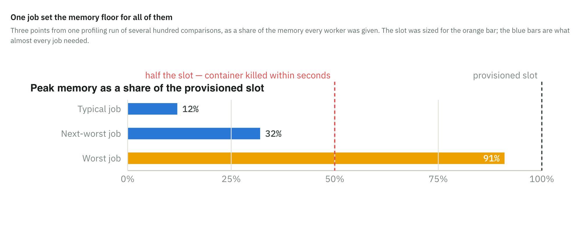
At eight bytes per entry, a table over a cluster in the high tens of thousands is several gigabytes on its own. Two of them, plus the working copies the library takes along the way, reached roughly fifteen gigabytes on the worst comparison we profiled.
That one comparison set the memory floor for every worker in the fleet. Every alignment job was provisioned at a slot large enough to survive it, roughly double what the typical job used. The worst case reached over ninety percent of that slot. Rerun at half the allocation, the container was killed within seconds of starting. Every job must be handed the same slot whether it needs one or not, so a node could hold half the workers the typical job would allow.
How We Found It
The cluster’s own metrics could not find it. Kubernetes reports container memory through the kubelet, scraped every few tens of seconds, per container. A spike that lives for a few seconds between two scrapes never appears. When a worker processes hundreds of jobs an hour, “this pod peaked at fifteen gigabytes at 14:32” narrows the search to a few hundred candidates and says nothing about which stage of any of them was responsible.
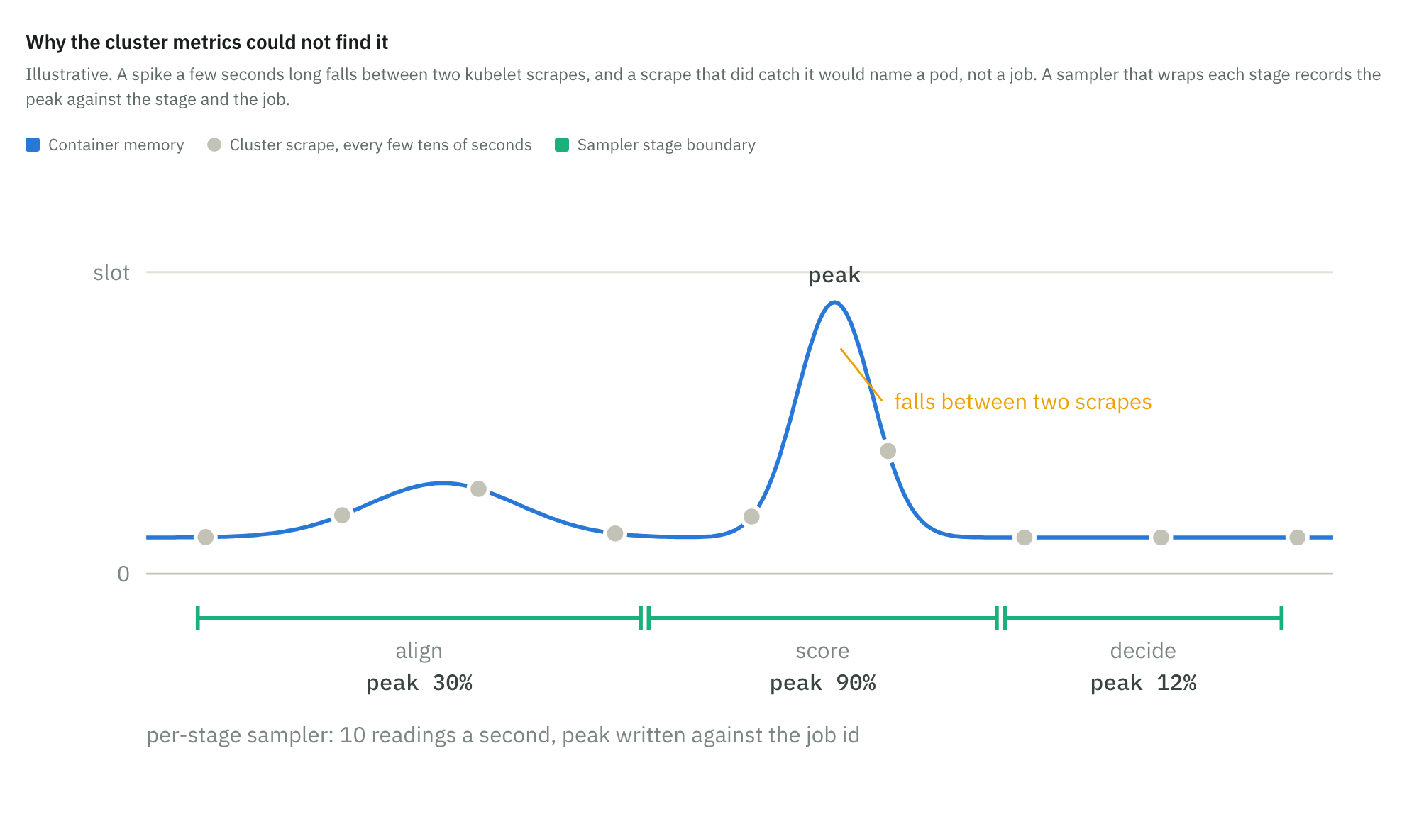
What broke the stalemate was instrumentation that attributed memory to a job and a stage rather than to a pod. We wrapped each stage of the pipeline in a sampler. It is a small thing. A background thread reads the container’s cgroup memory counter every hundred milliseconds for the duration of the stage, after a garbage-collection pass to fix a clean baseline. It records the peak, the mean and the delta against that baseline. The profile is written alongside the job’s result under the job’s own identifier, so every comparison carries its own memory history. “Which job, and which stage of it, needed fifteen gigabytes” becomes a query rather than an investigation.
Two properties of the sampler did the work. Ten-hertz sampling is fast enough to catch a spike the kubelet would miss. And attributing the reading to a stage boundary rather than a wall-clock timestamp let me say the problem was in scoring, not alignment. That turned a fleet-wide overprovisioning problem into one reproducible pair of scans and one function, and from there I could reproduce it with the scorer alone.
Four Ways To Bound A Square
There are only so many places to put a bound on a pairwise computation. You can shrink the input, shrink the sample, bound the allocation, or change the data structure. I implemented one of each behind a single switch and ran all four on the incident pair, ten repeats each, on the production node class.
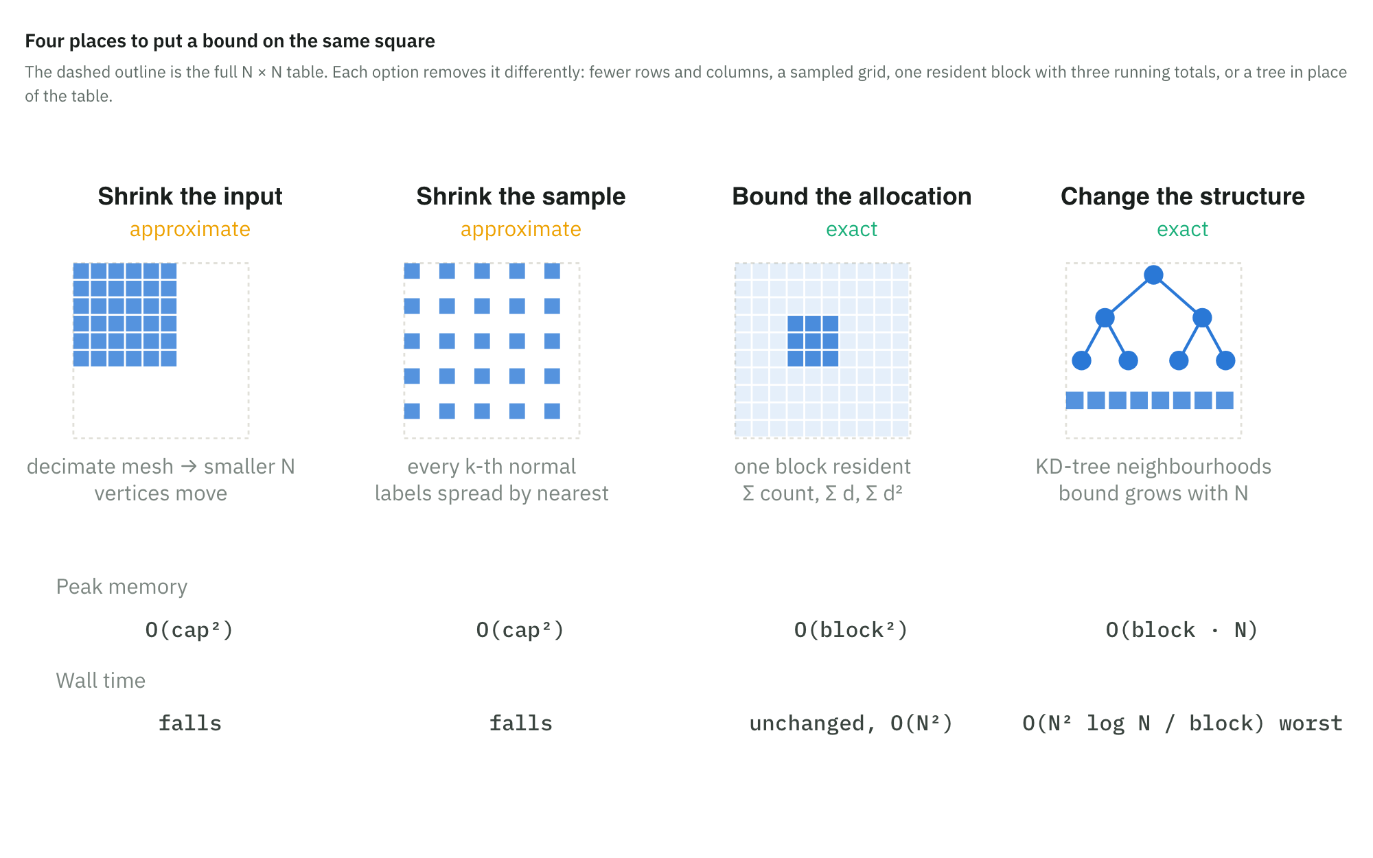
Shrink the input. Decimate the mesh at the top of the scorer when it exceeds a face budget. Every downstream step consumes the smaller mesh, so one gate bounds every quadratic site at once and everything gets faster. The cost is that decimation moves vertices. The geometry the scorer sees is no longer the geometry the scan recorded.
Shrink the sample. Take every k-th normal down to a fixed budget at evenly spaced indices. There is no random number generator, so the result is reproducible. Cluster the sample, then hand every unsampled normal the label of its nearest sampled neighbour. Memory is fixed by configuration rather than by the data: the table is budget-squared whatever N is. The result is an estimate, and a face at a cluster boundary can inherit the wrong label.
Bound the allocation. Never build the N × N table. Walk it in fixed-size blocks of rows, and for each block accumulate three running totals: the count of pairs, the sum of their distances, and the sum of their squares. The standard deviation falls out of those at the end. Peak memory is one block — a thousand rows square is eight megabytes. The number of distance evaluations is unchanged, so time stays quadratic. The work has not gone anywhere; it is just never all resident at once.
Change the structure. Index the normals in a KD-tree — a spatial search tree — so each neighbourhood query is bounded. Run the connected-components pass in blocks. Every face keeps its exact cluster label. The memory bound is linear in N rather than fixed, and the worst-case time on a near-complete neighbourhood graph is the price.
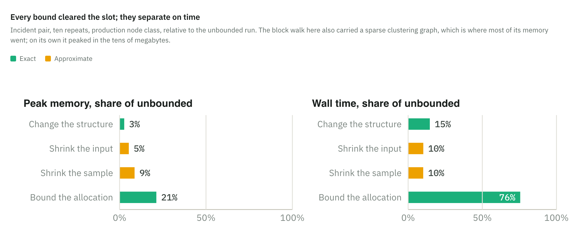
All four cleared the provisioned slot with room to spare, and they separate on two axes. On memory, the KD-tree was the most frugal, at roughly a thirty-seventh of the unbounded peak. Decimation and strided sampling came in at a nineteenth and an eleventh. The block walk, in the configuration I measured, came in at about a fifth. On time, the three modes that shrink something ran six to ten times faster than unbounded. The block walk ran at three-quarters of the original wall time, because it does the same number of distance evaluations.
Two things need saying before anyone reads that as a ranking. First, the block-walk row in that run also swapped the clustering step onto a sparse neighbours graph. That is where most of its memory went. The block walk on its own peaked in the tens of megabytes when I measured it in isolation. A sparse graph only helps when the graph is sparse, and near-parallel normals are exactly the case where it is not. Second, every mode produced a bit-identical alignment score on the incident pair. That sounds like proof and is not. On that pair the pyramid adjustment never fired, so the comparison could not exercise the path where a changed score would have changed the outcome.
What We Went With
We took two of the four forward to a load test on the production matching workload, across two datasets. The strided sample went because it was fast and nearest to the original code. The block walk went because it was exact. The single-pair run had bounded it without ever load testing it. The KD-tree mode had the best single-pair numbers and did not go, which is a gap I return to in the limitations.
Both candidates matched production on accuracy and precision on both datasets. Both cut the worst-case peak by more than eighty percent. Neither produced a single job above a quarter of the old slot, where production had produced dozens. That left latency, and latency pointed one way. Strided was about a fifth faster than production on the average matching job. Its slow tail improved more than its median. The block walk was about one percent slower than production, and its whole latency distribution sat on top of production’s. That is exactly what the design predicts. Streaming changes where the memory goes, not how much work is done.
We shipped the block walk anyway, and the reason is the arithmetic.
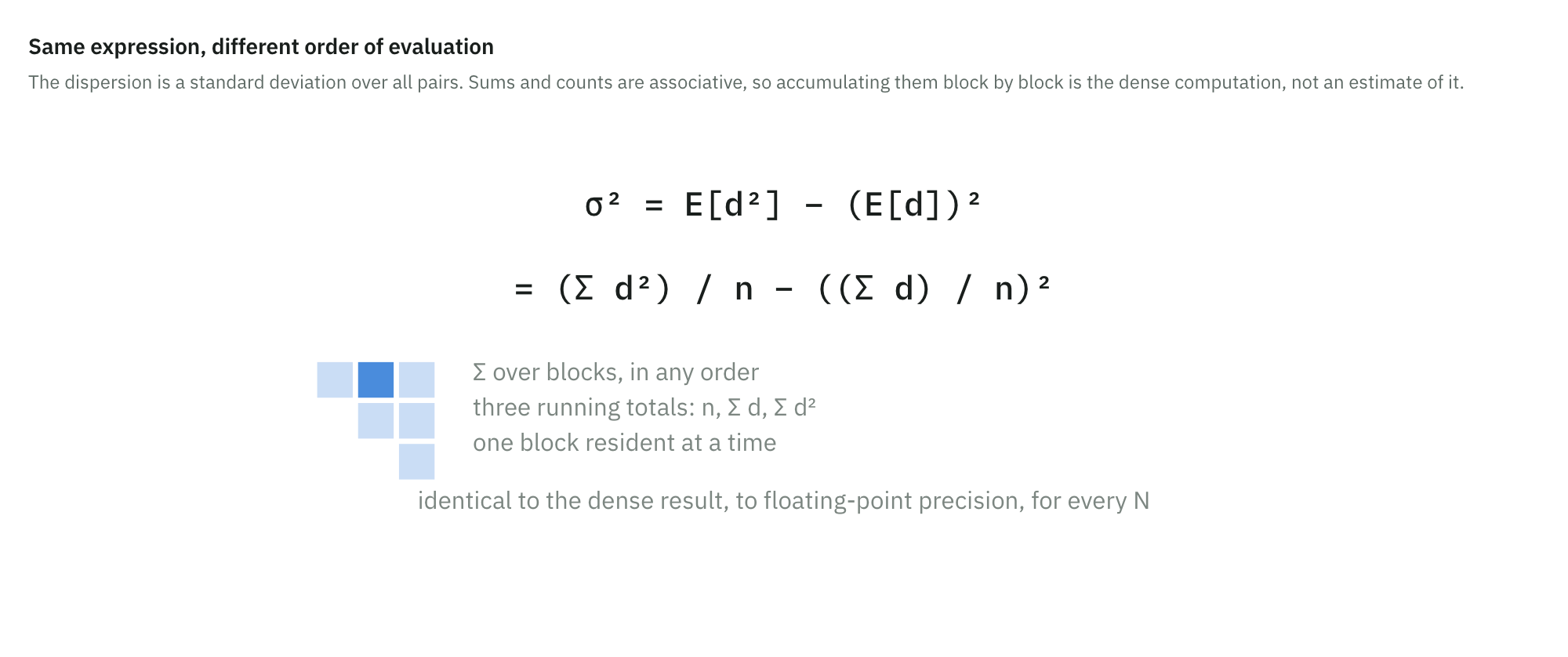
The scorer required of each pairwise distance. To compute this we required:
-
the count of the distances
-
their sum and the squared sum
Those three totals can be built up in any order and any grouping and come out the same. The block based approach therefore computes the same expression in increments. Therefore it is an closed-form alternative to the original approach with the same behaviour and guarantees.
Strided is an approximation. Its error was negligible on two datasets which didn’t say enough about production. Given the system audits supply chains, we went for a safer exact solution rather than one that changed the problem with limited coverage.
Where Else This Could Surface
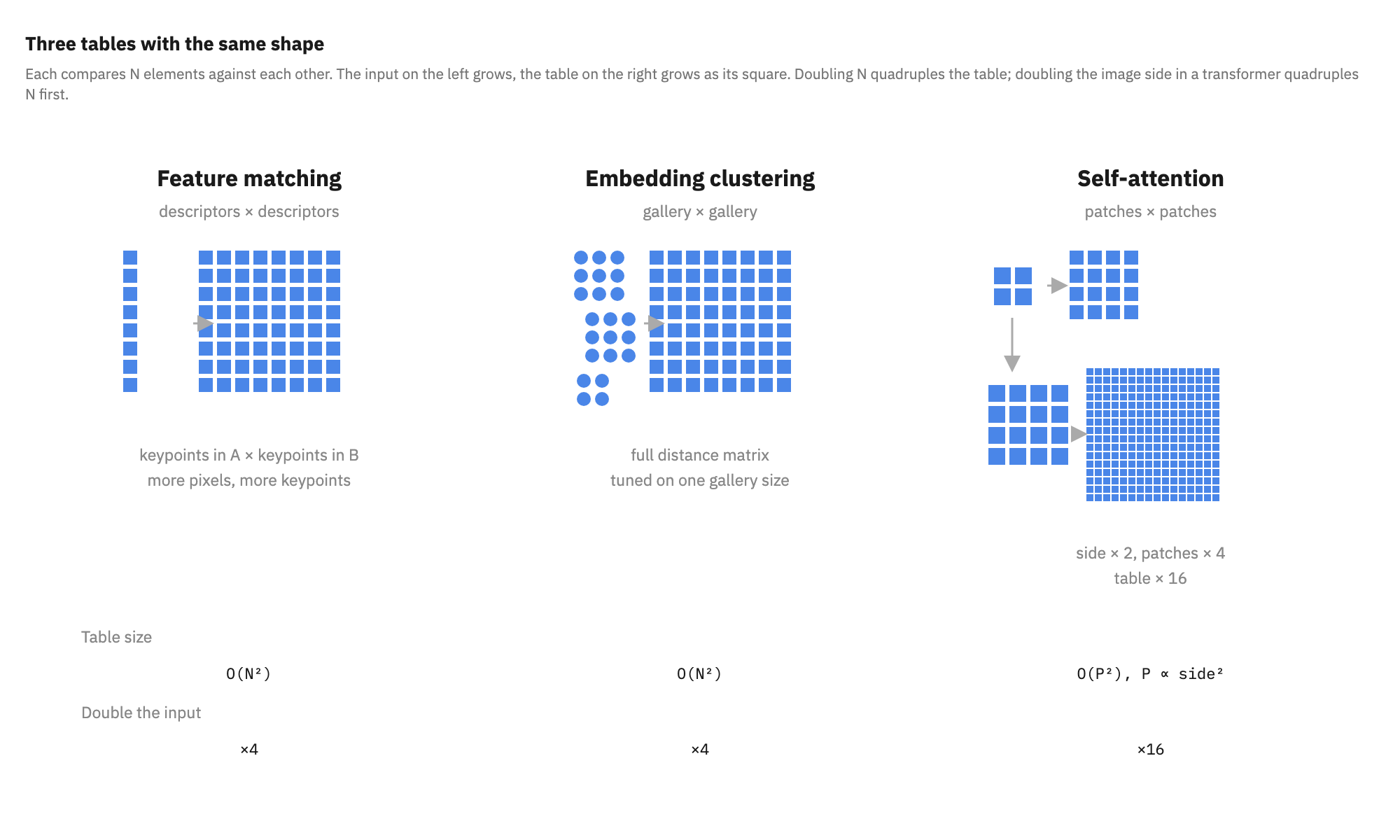
The square appears wherever an algorithm compares elements to each other. Compare each of N items against k others at a time and the table is N to the power k plus one. Pairs give N squared. Triples give N cubed. The dispersion table was the pairs case, and that was enough.
-
Feature matching. Two images, a descriptors-by-descriptors distance table. A higher-resolution image does not add features linearly.
-
Embedding clustering. Re-identification, deduplication, anything that wants a full distance matrix. It is tuned on a gallery of one size and fails when the gallery grows past it.
-
Self-attention in a vision transformer. The pizza problem twice over. Doubling the image side quadruples the patch count, and the attention table is the square of that. Sixteen times the memory for an image that looks twice as big.
Bounding these share the same set of solutions, including:
-
shrink the inputs and pay a resolution cost
-
subsample and pay an approximation cost
-
compute in blocks and pay a time overhead
-
index the space and (maybe) end up where you started
The input that blew up production was the dense one.
Conclusion
Faced with a similar problem, here are two things I’d do differently.
Pay attention to any output with more dimensions than its input. A function that takes N things and returns N-by-N things is a quadratic site. This always should be flagged and measured against the worst N. In our codebase the docstring said nothing about allocations. The square was in plain view for a year because everyone read the signature and saw a list.
Decide up front what we are willing to pay. Every bound costs something: fidelity, an approximation, wall time, or a data-dependent worst case. We decided at experimentation which of these would be worth sacrificing. In reality we were happy to tolerate a small time increase in the worst case. Deciding this up front would have removed the experimentation with approximation methods as viable candidates.