Three Samplers, One Posterior: NUTS vs. Emcee vs. Nested Sampling

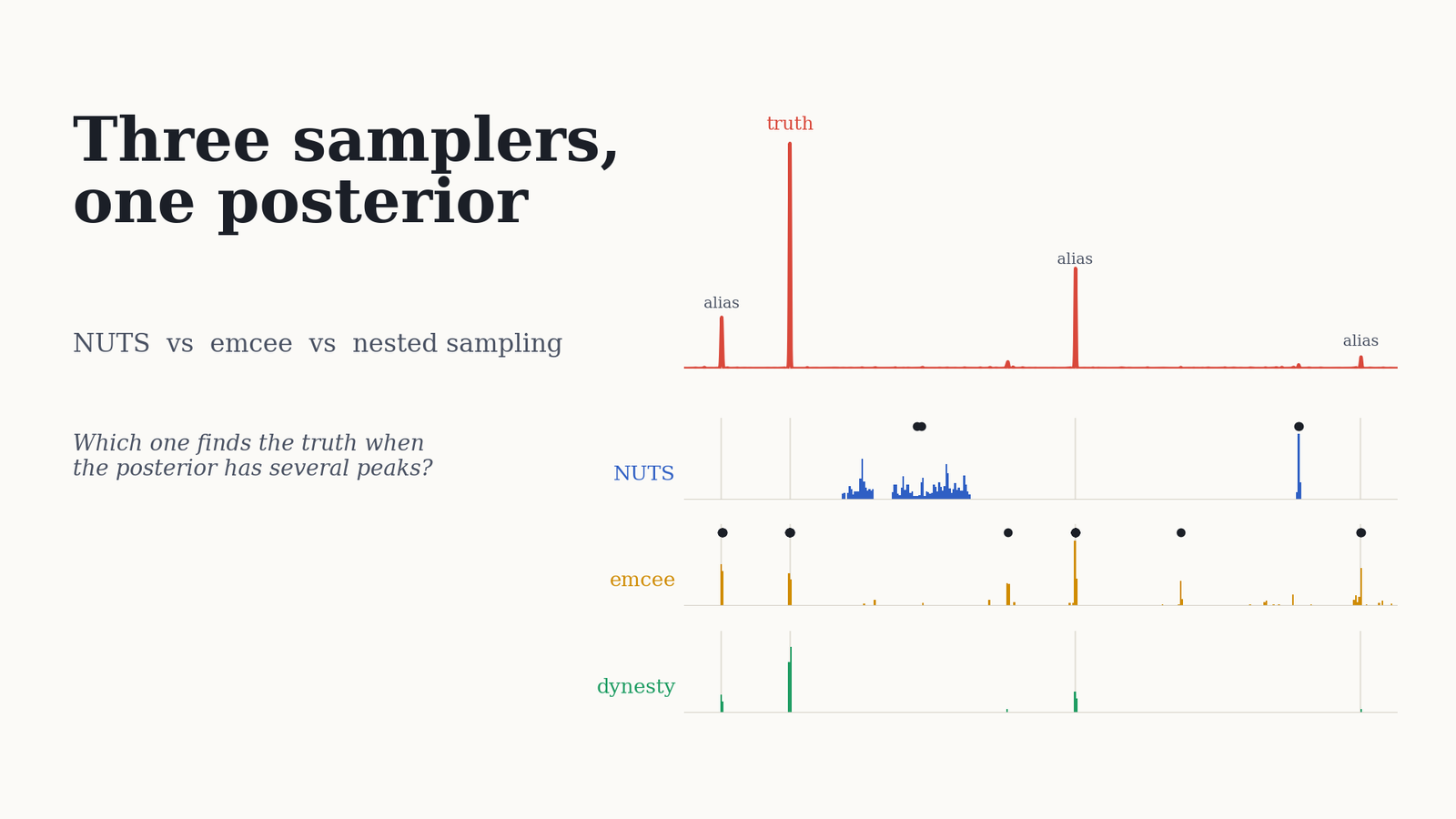
I’ve used all three of these samplers in actual research, usually without thinking much about why I picked one over another. emcee was the sampler I first used. NUTS came along when I moved my likelihoods to JAX. dynesty came out whenever someone asked for a Bayes factor. At some point I realised I couldn’t actually say which one I’d trust on a problem I didn’t already understand.

The trouble with most sampler comparisons is that they measure speed, and speed is meaningless if the samples are wrong. You can only check “wrong” when you know the right answer. So I picked three problems small enough to solve exactly, either on a dense grid or analytically, and scored each sampler against the truth rather than against the other samplers.

In Short

NUTS was the fastest by a factor of two to four on smooth problems. On the multimodal problem it failed completely, and its diagnostics said so very clearly.

emcee was fine on the easy problems. On the multimodal one it gave confidently wrong answers, and nothing in its default output warned me.

dynesty was the only one that found every mode and the only one that produced a correct evidence. Its error bars on the evidence turned out to be optimistic, though.

The setup I use

A quick word on what each sampler actually does, because it explains almost everything that follows. NUTS is Hamiltonian Monte Carlo with an automatic choice of trajectory length. It uses gradients of the log-posterior to glide along the surface. I ran it through NumPyro, which sits on JAX. emcee runs an ensemble of walkers using the Goodman–Weare stretch move, and needs no gradients at all. dynesty does nested sampling: it starts from the whole prior and steadily shrinks towards higher likelihood, using a set of overlapping ellipsoids to keep track of where the live points are.

The three test problems get progressively harder.

P1, the control. Fit Ω_m and H₀ in flat ΛCDM to 40 simulated Type Ia supernovae. A nice, roughly elliptical posterior.

P2, the banana. Same supernovae, but fit Ω_m and the dark energy equation of state (w) with H₀ held fixed. Supernovae alone can’t separate those two, so the posterior is a long, thin, curved ridge.

P3, the multimodal one. Find the frequency of a sinusoid observed on 40 nights spread over 80 days. Because the observations are about a day apart, the posterior has several separated peaks. More on why below.

Each sampler got identical uniform priors and the identical likelihood. For NUTS I used 4 chains with 1000 warm-up and 2000 kept draws each. For emcee, 32 walkers for 6000 steps, throwing away the first 1500. For dynesty, 1000 live points with bound='multi', sample='rwalk' and dlogz=0.01. emcee and dynesty both started from the prior, not from a best fit, since I wanted to see whether they’d find things on their own.

Effective sample size and R̂ for NUTS use the rank-normalised versions in ArviZ. For emcee I took ESS from its integrated autocorrelation time, and for dynesty from Kish’s formula on the importance weights.

For the P3 reference, two amplitudes enter the model linearly, so they can be integrated out exactly at each frequency:

p(f | y) ∝ 2π · det(X_f^TX_f/σ²)^−1/2 · exp[−½ χ²_min(f)]

I evaluated that on 40,000 frequencies, which gives the exact mode weights and the exact evidence.

Everything ran on CPU on my laptop, with NumPyro 0.19, JAX 0.6, emcee 3.1 and dynesty 3.0.

Problem 1: the easy one

No surprises. All three land on the right answer, with the right width. NUTS is about twice as efficient, but I’d give most of the credit for that to JAX compiling the likelihood and its gradient, not to anything clever NUTS is doing. If your problem looks like this one, just use whatever you’re comfortable with.

Problem 2: the banana shape

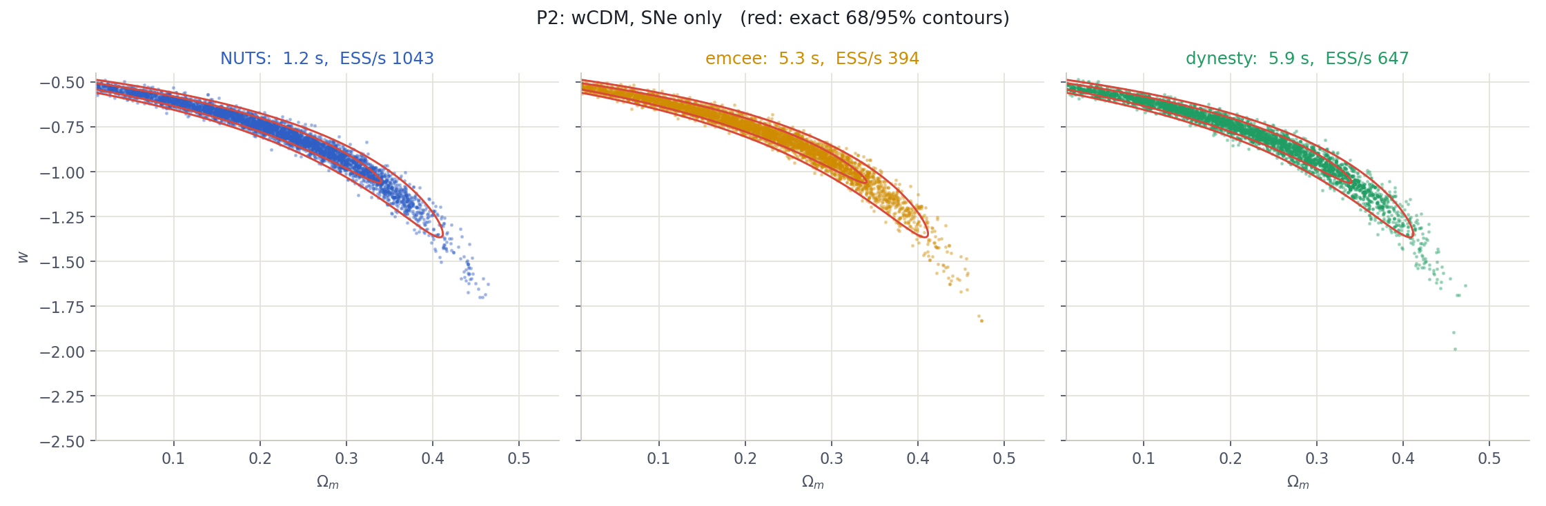
I expected at least one sampler to struggle here, and none really did. All three still match the exact contours. What changes is how much each one has to work for it.

emcee took the biggest hit. Its stretch move is affine-invariant, which means it copes with straight-line correlations for free. A curved ridge isn’t a straight line, so walkers keep proposing points that fall off the edge of the banana, and the acceptance rate drops from 0.72 to 0.62. NUTS slowed down too, for a related reason: the mass matrix it adapts during warm-up is a single linear rescaling and can’t follow the bend, so it needs roughly twice as many gradient evaluations (63k up to 116k). dynesty barely noticed. Nested sampling only cares about how the likelihood contours shrink, and a set of ellipsoids can wrap a banana quite well.

Remember not to read too much into this round. In two dimensions a banana is mostly an inconvenience. In twenty dimensions with several of them, I’d expect emcee to go from slow to genuinely broken, since ensemble samplers are known to degrade quickly with dimension. If NUTS is the one struggling, the usual fix is to reparameterise so you’re sampling along the ridge, and only then reach for a dense mass matrix.

Problem 3: the multimodal one

This is where things got interesting.

First, what an alias is

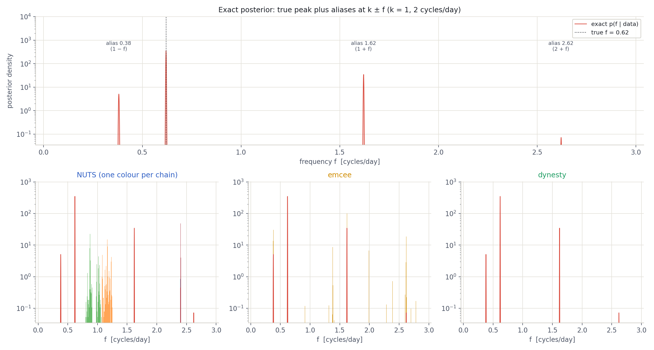
If you only observe a star once a night, at about the same time each night, your observations are spaced almost exactly one day apart. Now picture a sine wave at frequency f, and a second one at f + 1 cycles per day. Between two observations the second wave goes round one extra full cycle, and so on the nights you actually look, the two waves have exactly the same value. You simply can’t tell them apart. The same is true for f + 2, f + 3 and so on, and also for 1 − f, which is the same wave reflected to negative frequency.

In this problem the true frequency is 0.62 cycles per day. That puts the aliases at:

• 1.62 c/d, which is 1 + f, the true signal plus one extra cycle per day,

• 0.38 c/d, which is 1 − f, the mirror image of the true signal,

• 2.62 c/d, which is 2 + f, two extra cycles per day.

The only thing that breaks the tie is the small night-to-night scatter in when the observations happen (about an hour and a half here). So the aliases fit the data nearly as well as the truth. They aren’t artefacts of any sampler; they’re real, smaller peaks in the posterior. In the exact answer, 89% of the probability sits on the true peak, 9% on the 1.62 alias and 2% on the 0.38 alias.

What the samplers did

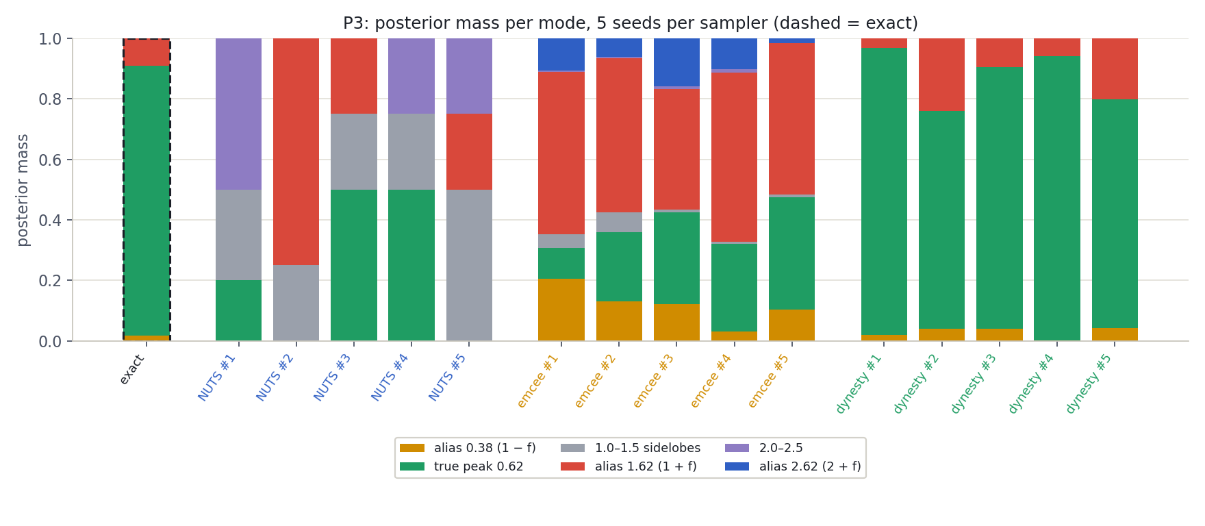
One run can be a fluke, so I ran each sampler five times with different seeds on the same data.

NUTS. Every chain simply got stuck on whatever bump in the likelihood was nearest to where it started. Some of those bumps weren’t even aliases, just small sidelobes of the periodogram. In hindsight this is obvious. A gradient tells you which way is uphill from where you’re standing, and nothing about a taller hill a long way off. The silver lining is that the failure was impossible to miss: R̂ above 2 and an effective sample size of about 5 on every single run. (One caveat about the table: NUTS’s “true peak” number includes chains stuck on a sidelobe near 0.87, which happens to fall in the same window, so it actually flatters NUTS.)

emcee. This is the result that bothered me most. The walkers did find real modes, but they put about half of the probability on the 1.62 alias, which should get 9%. And they did it consistently, with only a few percent of scatter between runs, so rerunning with a new seed wouldn’t have tipped me off. The only hint was emcee’s own note that the chain was shorter than fifty autocorrelation times. The underlying reason is that walkers can only hop between modes when a stretch move happens to land on the other one, which almost never happens, so they stay wherever they settled during burn-in.

dynesty. It found all three modes and, averaged over the five runs, got their weights right. Any single run, though, could be off by about ten percentage points in how it split the probability. If the ratio between modes is actually your science result, I’d combine several runs or increase the number of live points.

What it all cost

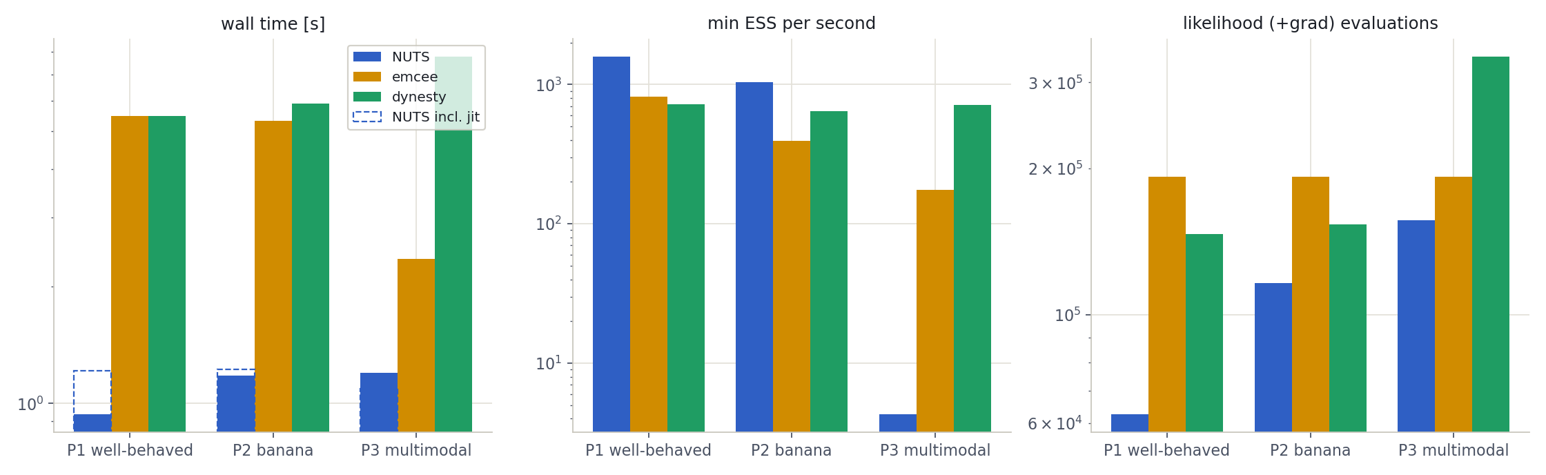
On the two smooth problems NUTS was four to six times quicker in wall time. JIT compilation only added a fraction of a second here because the models are tiny; on a real pipeline it can be tens of seconds, which matters for a quick fit and doesn’t matter at all if you’re running the same model a thousand times.

In fairness to emcee and dynesty, I gave them a plain numpy likelihood that they call one point at a time, so they pay Python overhead on every evaluation. Vectorising the likelihood would close some of the gap. NUTS mostly wins because JAX hands it compiled gradients for free.

The evidence

If you want to compare models with Bayes factors, you need the evidence, Z = ∫ 𝓛(θ) π(θ) dθ. Nested sampling is built around computing it. MCMC samples, on the other hand, don’t contain any direct information about Z.

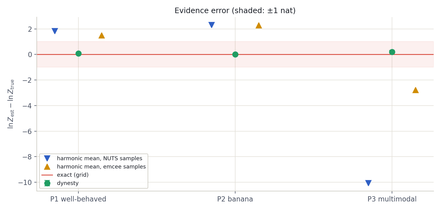
The tempting workaround is the harmonic-mean estimator, which only needs the likelihood at your posterior samples. Radford Neal once called it the worst Monte Carlo method ever, and these runs show why:

dynesty lands within about 0.2 of the exact value every time. The harmonic mean is off by 1.5 to 2.3 even on the easy problems, which is more than enough to flip a model comparison, and by 3 to 10 on the multimodal one.

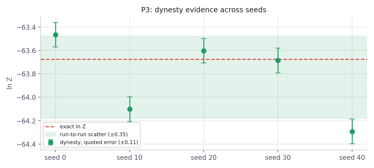
There’s one catch, which only showed up in the repeated runs. Across five runs on P3, dynesty’s estimates centred nicely on the truth (−63.83 against −63.67), but they scattered by ±0.35, while each run reported an uncertainty of only ±0.11. On a multimodal problem I’d now treat dynesty’s quoted error as optimistic by a factor of a few, and get a real error bar by running it more than once.

So which one should you use?

Here’s roughly how I’d decide now, in the order I’d ask the questions.

Do you need the evidence, for model comparison? Use dynesty. Nothing else here gives you a number you can trust.

Is there any chance of more than one mode? Periodograms, mixture models, label switching and strong lensing are the usual suspects. Use dynesty here too. The other two only find the modes they happen to start near.

Can you write the model in JAX, and is it smooth with a single peak? Use NUTS. It’s the most efficient by a wide margin, it scales to hundreds of parameters, and R̂ and divergences will tell you when it’s in trouble.

Is there a curved degeneracy? NUTS is still a good choice, but reparameterise first. dynesty is the fallback.

Is your likelihood a black box, say a Fortran code or a simulator, with ten or fewer parameters and a posterior you’re confident has one peak? emcee is perfectly good. It needs no gradients, the API is tiny and it parallelises trivially.

A combination I’ve ended up using a lot: run dynesty once to map out the posterior and get the evidence, then run NUTS inside the mode you care about for the high-quality samples.

Three habits that would have caught every failure

First, run at least four chains from spread-out starting points and actually look at R̂. That alone caught NUTS.

Second, never take an emcee result without checking the autocorrelation time. If the chain isn’t at least fifty autocorrelation times long, you don’t have a posterior yet.

Third, before trusting any sampler on your real problem, try it on a version you can solve exactly. A two-dimensional grid takes seconds, and it’s the only way to find out what “correct” looks like.

···

How the likelihood is shared between the three

The fairness of a comparison like this depends on every sampler seeing exactly the same likelihood. The awkward part is that they want it in different forms. NUTS needs gradients, so NumPyro wants the model written in jax.numpywhere it can differentiate it. emcee and dynesty don’t care about gradients and just call a plain Python function that returns a number. Here is the P1 supernova likelihood both ways, cut down to the essentials.

The physics, the distance modulus from a cumulative trapezoid integral of 1/E(z), is written twice: once in NumPy and once in JAX. The two versions are line-for-line identical apart from the np/jnp prefix:

import numpy as npimport jax.numpy as jnpdef distmod(Om, w, H0):                 # NumPy: for emcee and dynesty    zp = 1 + zgrid    invE = 1 / np.sqrt(Om * zp**3 + (1 - Om) * zp**(3 * (1 + w)))    dc = np.concatenate([[0.], np.cumsum(0.5 * (invE[1:] + invE[:-1]) * dz)])    return 5 * np.log10((1 + zsn) * dc[isn] * c_kms / H0) + 25def distmod_jax(Om, w, H0):             # JAX: same maths, differentiable for NUTS    zp = 1 + zgrid    invE = 1 / jnp.sqrt(Om * zp**3 + (1 - Om) * zp**(3 * (1 + w)))    dc = jnp.concatenate([jnp.zeros(1), jnp.cumsum(0.5 * (invE[1:] + invE[:-1]) * dz)])    return 5 * jnp.log10((1 + zsn) * dc[isn] * c_kms / H0) + 25

For NumPyro, you don’t write a log-likelihood function at all. You describe the generative model, and the priors and the Gaussian likelihood become samplestatements. NumPyro builds the log-density and its gradient from that:

import numpyroimport numpyro.distributions as distfrom numpyro.infer import MCMC, NUTSdef model():    Om = numpyro.sample("Om", dist.Uniform(0.05, 0.6))    H0 = numpyro.sample("H0", dist.Uniform(55., 85.))    numpyro.sample("obs", dist.Normal(distmod_jax(Om, -1.0, H0), sig), obs=mu_obs)mcmc = MCMC(NUTS(model), num_warmup=1000, num_samples=2000, num_chains=4)mcmc.run(jax.random.PRNGKey(0))

For emcee and dynesty, the same Gaussian likelihood is a few lines of NumPy. The one thing that changes between them is where the prior lives. emcee wants a log-posterior, so the uniform prior goes in as a hard boundary that returns −∞. dynesty never evaluates the prior; it asks for a transform from the unit cube to parameter space and samples the prior directly:

import emcee, dynestylo, hi = np.array([0.05, 55.]), np.array([0.6, 85.])def loglike(theta):    Om, H0 = theta    r = mu_obs - distmod(Om, -1.0, H0)    return -0.5 * np.sum(r**2) / sig**2 - len(r) * np.log(sig * np.sqrt(2 * np.pi))def logpost(theta):                     # emcee    return loglike(theta) if np.all((lo <= theta) & (theta <= hi)) else -np.infdef prior_transform(u):                 # dynesty    return lo + u * (hi - lo)p0 = lo + np.random.rand(32, 2) * (hi - lo)          # walkers drawn from the prioremcee.EnsembleSampler(32, 2, logpost).run_mcmc(p0, 6000)dynesty.NestedSampler(loglike, prior_transform, 2, nlive=1000,                      bound="multi", sample="rwalk").run_nested(dlogz=0.01)

Two small things are worth knowing if you try this yourself. First, keep the normalising constant (the len(r) * np.log(...) term) in the likelihood. MCMC doesn’t care about it, but the evidence does, and dropping it would shift every ln Z in the table above. Second, before running anything, check that the two versions agree: evaluate distmod and distmod_jax at a few random points and confirm they match to machine precision. It takes a minute and rules out the most embarrassing kind of sampler “disagreement”.

···

References

1. Hoffman, M. D. & Gelman, A. (2014). The No-U-Turn Sampler: adaptively setting path lengths in Hamiltonian Monte Carlo. JMLR 15, 1593–1623. arXiv:1111.4246

2. Neal, R. M. (2011). MCMC using Hamiltonian dynamics. In Handbook of Markov Chain Monte Carlo, CRC Press. arXiv:1206.1901

3. Betancourt, M. (2017). A conceptual introduction to Hamiltonian Monte Carlo. arXiv:1701.02434

4. Phan, D., Pradhan, N. & Jankowiak, M. (2019). Composable effects for flexible and accelerated probabilistic programming in NumPyro. arXiv:1912.11554

5. Bradbury, J. et al. (2018). JAX: composable transformations of Python+NumPy programs. github.com/jax-ml/jax

6. Foreman-Mackey, D., Hogg, D. W., Lang, D. & Goodman, J. (2013). emcee: the MCMC hammer. PASP 125, 306. arXiv:1202.3665

7. Goodman, J. & Weare, J. (2010). Ensemble samplers with affine invariance. Comm. App. Math. Comp. Sci. 5, 65–80. doi:10.2140/camcos.2010.5.65

8. Speagle, J. S. (2020). dynesty: a dynamic nested sampling package for estimating Bayesian posteriors and evidences. MNRAS 493, 3132. arXiv:1904.02180

9. Skilling, J. (2006). Nested sampling for general Bayesian computation. Bayesian Analysis 1, 833–859. doi:10.1214/06-BA127

10. Feroz, F., Hobson, M. P. & Bridges, M. (2009). MultiNest: an efficient and robust Bayesian inference tool for cosmology and particle physics. MNRAS 398, 1601. arXiv:0809.3437

11. Riess, A. G. et al. (1998). Observational evidence from supernovae for an accelerating universe and a cosmological constant. AJ 116, 1009. arXiv:astro-ph/9805201

12. Perlmutter, S. et al. (1999). Measurements of Ω and Λ from 42 high-redshift supernovae. ApJ 517, 565. arXiv:astro-ph/9812133

13. VanderPlas, J. T. (2018). Understanding the Lomb–Scargle periodogram. ApJS 236, 16. arXiv:1703.09824

14. Vehtari, A., Gelman, A., Simpson, D., Carpenter, B. & Bürkner, P.-C. (2021). Rank-normalization, folding, and localization: an improved R̂ for assessing convergence of MCMC. Bayesian Analysis 16, 667. arXiv:1903.08008

15. Kumar, R., Carroll, C., Hartikainen, A. & Martin, O. (2019). ArviZ: a unified library for exploratory analysis of Bayesian models in Python. JOSS 4, 1143. doi:10.21105/joss.01143

16. Sokal, A. (1997). Monte Carlo methods in statistical mechanics: foundations and new algorithms. In Functional Integration, Springer, 131–192. doi:10.1007/978-1-4899-0319-8_6

17. Higson, E., Handley, W., Hobson, M. & Lasenby, A. (2019). Dynamic nested sampling: an improved algorithm for parameter estimation and evidence calculation. Statistics and Computing 29, 891. arXiv:1704.03459

18. Newton, M. A. & Raftery, A. E. (1994). Approximate Bayesian inference with the weighted likelihood bootstrap. JRSS B 56, 3–48. doi:10.1111/j.2517-6161.1994.tb01956.x

19. Neal, R. M. (2008). The harmonic mean of the likelihood: worst Monte Carlo method ever. Blog post. radfordneal.wordpress.com

20. Gelman, A. & Rubin, D. B. (1992). Inference from iterative simulation using multiple sequences. Statistical Science 7, 457–472. doi:10.1214/ss/1177011136