

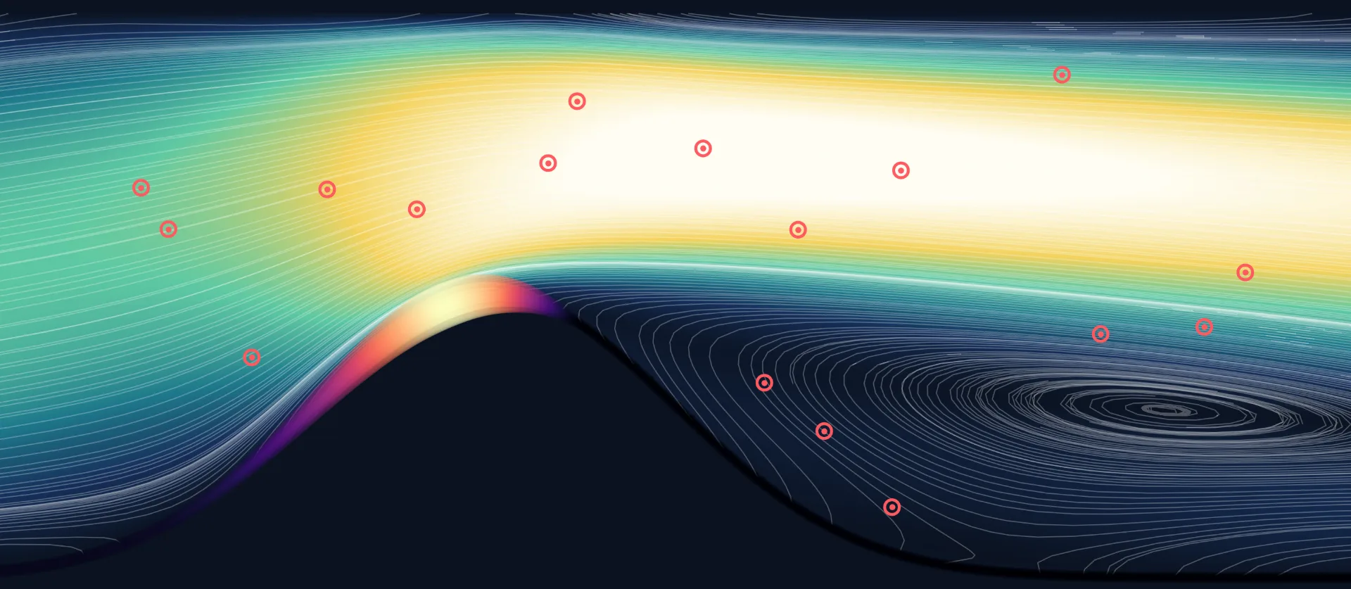
Wall shear stress is the friction blood puts on the wall of a vessel. It is tied to where plaque builds up, and it is hard to measure directly. What a clinic can get, with Doppler ultrasound for example, is the velocity at a few points inside the vessel. So the question for this article is whether a neural network can take those scattered, noisy velocities, together with the equations of fluid flow, and give back the whole flow field and the shear stress at the wall.
A physics-informed neural network (PINN) is a natural fit. I built one in plain PyTorch, without DeepXDE or any other PINN library, for a 2D artery with a narrowing (a stenosis). From 40 velocity readings it reconstructs the velocity and pressure fields and the region of reversed flow behind the narrowing. It also works out the viscosity of the fluid, which I treated as unknown, and its wall shear stress follows the CFD reference closely.
This is the first article in a series about PINNs for blood flow. It covers the core: the Navier-Stokes residual, a learnable viscosity, and what decides whether the result is any good. Later articles cover the CFD solver behind the reference data and a pulsating flow that follows a heartbeat.
The Setup
The artery is a 2D channel of height H with a smooth bump on the lower wall that blocks half of the opening, a 50% stenosis. The flow is incompressible Navier-Stokes at a Reynolds number of 200, with lengths measured in channel heights and velocities in inlet velocities. That is a slow flow, at the low end of what happens in a carotid artery. In these units the kinematic viscosity is 0.005.
There are no patients in this article, on purpose. To score a reconstruction you need to know the right answer, so I generated it. A Navier-Stokes solver I wrote (a projection method on a staggered grid) computes the steady flow, and the PINN only ever gets a few noisy readings taken from that solution. The noise is Gaussian, at 7% of the inlet velocity. I might cover the solver in a later article.
The length of the channel mattered more than I expected. My first version was five heights long. Behind the bump the flow separates from the wall and a region of reversed flow forms. In five heights that region never closed: fluid was still moving backwards at the outlet, where the solver assumes it leaves. The outlet was shaping the reference solution as much as the physics was. Stretching the channel to nine heights fixed it. The reversed flow now ends around x = 5.8 and everything after that runs forward.
The readings are 40 points inside the fluid, each with a velocity vector plus noise. There are no pressure readings and no readings right at the wall. I placed them in four bands along the channel, with more of them around the throat and the wake than near the inlet and outlet. That layout made little difference, which I come back to at the end.
The network is a plain MLP with 6 layers of 32 tanh units, about 5,500 weights. It uses tanh because the momentum equation needs second derivatives of the output, and the second derivative of a ReLU is zero almost everywhere. The inputs are rescaled to the range -1 to 1 inside the network, so autograd still differentiates with respect to the physical coordinates.
Writing the Navier-Stokes residual in PyTorch
A PINN maps coordinates to physical quantities. Here that is (x, y) -> (u, v, p): two velocity components and the pressure. The loss has a term that fits the measurements, like any regression, and a term built from the residual of the equations: how badly the network’s own output violates them. You get the residual by differentiating the network with respect to its inputs, which is what autograd is for. For incompressible Navier-Stokes there are three of them, continuity and one momentum equation per velocity component.
If those three are close to zero at points scattered over the channel, the network is close to a solution of the equations, and the sensors pick out which one. The viscous term needs u_xx, a derivative of a derivative, so autograd has to keep the graph of the first derivative around. That is what create_graph=True does. Leave it out and the second call fails in the first epoch.
The loss adds up three groups, each with a weight:
-
data, with weight 100, is the squared error against the 40 readings -
pde, with weight 10, are the three residuals at 2,500 points spread over the fluid -
bc, with weight 10, no-slip on both walls, are the inlet profile, and the outflow condition (zero pressure and zero streamwise gradient at the outlet)
The pde weight was the first thing I got wrong. At a weight of 1 the physics term was too small to shape anything, and the velocity error came out more than twice as large as with 10. A weight of 50 did about the same as 10. The collocation points are resampled every 200 epochs, and 30% of them are picked where the residual is currently largest. Training is Adam for 10,000 epochs with a decaying learning rate, followed by 400 iterations of L-BFGS, which took around 35 minutes on three CPU threads.
Making viscosity a learnable parameter
In a forward problem you know all the physics and want the field. Here the viscosity is unknown, so it becomes one more parameter, optimized alongside the network weights. It only appears in the residual, as the number multiplying the second-derivative terms. I store its logarithm, which keeps it positive and puts it on a scale where an Adam step is reasonable for a number as small as 0.005.
What do you start it at? In practice you would use a literature value for blood, and that is a fine starting point. Here I wanted to check that the answer comes from the sensors and not from where the parameter began, so I started far away. One run started at four times the true value, another at about a third of it. Both ended close to the truth.
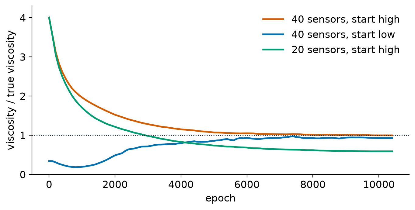
That last curve is the one to look at. Viscosity only reaches the loss through the physics term, and the physics term only means something once the velocity field is roughly right, so early in training the parameter moves erratically and later it settles. What it settles on depends on how much the data constrain the flow. With 20 sensors it went to the wrong value every time I tried, in every variant of the learning rate and loss weights: between a quarter and a half off, sometimes high and sometimes low, with loss curves that looked healthy the whole way. My reading is that twenty noisy points cannot tell “thicker fluid, smoother flow” from “thinner fluid, sharper flow”, so the network picks one of them.
With 40 sensors, and everything else the same, viscosity landed on the right value. Changing the learning rate did far less than adding data, which is not the answer I expected when I started tuning it.
Results
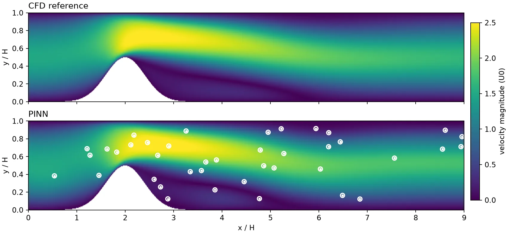
The reconstructed velocity field is within a few percent of the CFD field, about what I’d expect from readings with this much noise in them. The v component alone looks worse in relative terms, because the flow is mostly axial and the same absolute error is divided by a much smaller number.
A velocity map can look right while the flow structure is off, so I also compared vorticity, the local rotation of the fluid. The interesting part of this flow is the layer of strong shear between the fast jet and the slow reversed-flow zone, and how it fades downstream.
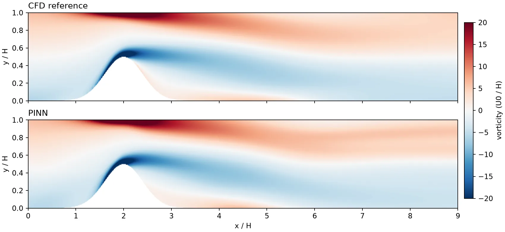
The reversed-flow region is reproduced too. In the CFD it starts at x = 2.2 and closes at about x = 5.75. In the PINN it starts at the same place and closes at about x = 5.6. No sensor sits on the wall, so that comes from the physics working together with the readings.
The recovered viscosity in this run was 0.00498 against a true 0.005, which is a little better than typical. It was the first run with 40 sensors. The other runs with 40 or more sensors, with different starting points and different random draws of the sensors, ended between 1% and 8% off.
For wall shear stress, which is what the exercise was for, the PINN’s curve follows the reference.
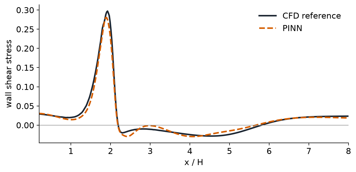
It has the right shape everywhere, and its peak comes out a little low. One note on the reference. The solver’s staircase-shaped wall makes a raw finite-difference estimate of the wall gradient jagged. For both the CFD field and the network I instead take the velocity along the wall normal at a few points a short distance from the wall and fit the gradient through them, using the fact that the velocity is zero at the wall. Both curves are read the same way.
What made the difference
Since the sensors mattered most, here is what I varied around the 40-sensor run. All of these used the same network and training.
|
Change |
Effect |
|---|---|
|
20 sensors instead of 40 |
viscosity a quarter to a half off; velocity error the same or worse |
|
60 sensors |
about the same as 40 |
|
40 sensors spread uniformly, not in bands |
slightly worse vorticity, viscosity within about 8% |
|
no outflow condition |
about the same |
|
wider network (4 layers of 96) |
no better, about twice as slow |
|
|
velocity error more than twice as large |
Scaling the inputs, decaying the learning rate and picking collocation points by residual made little difference to the velocity error when I tried them on the first channel. I kept them because they cost almost nothing. The outflow condition changed little, so if you would rather not tell the network about your outlet, you can leave it out here.
Most of the improvement came from the data: enough sensors to pin the viscosity down, and a channel long enough that the outlet stayed out of the way. The architecture and optimizer settings I tried moved things much less.
Where this stops
The flow is 2D and steady, the walls are rigid, and the noise is plain Gaussian noise, which stands in for a Doppler measurement without modeling beam angle or speckle. Forty probes placed wherever I chose is also a generous setup compared with a real exam. The results come from one geometry at one Reynolds number.
Blood is also shear-thinning, so a constant viscosity is least accurate in the slow, separated zone behind the stenosis, right where the reversed flow sits. And the link between wall shear stress and plaque, while well studied, is still argued about.
The next article is about the CFD solver that produced the reference data, including a bug in my wall-shear-stress reference that made a good result look bad. All code, configs and figures are in the repo: [link].