How Wrong Is Your Marketing Mix Model (MMM)?

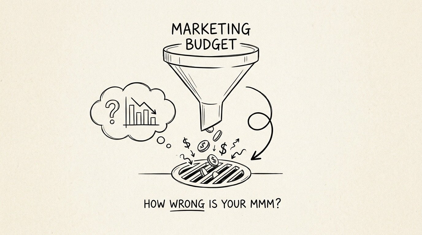
Measuring the return on marketing spend is one of the hardest jobs in growth, but Marketing Mix Modelling has had a resurgence as the answer to it in recent years. Open-source releases have driven most of that: Robyn from Meta, Meridian from Google, PyMC-Marketing from PyMC Labs. Running an MMM has never been easier. Trusting one is a different question.

Google set out why back in 2017, in Challenges and Opportunities in Media Mix Modeling, a paper that is still the clearest statement of what goes wrong. Three of the problems it names do most of the damage. Each one comes from a different kind of variation that is missing from your spend.

• Multi-collinearity. Marketing channels get set in the same planning cycle, so they rise and fall together. No model can separate channels that never moved apart, so the estimates come back with high variance. What is missing is each channel moving on its own.

• Selection bias. Spend follows demand, with organisations spending more on marketing in peak periods. But as demand itself isn’t directly observable, the model has to fall back on proxies for it. The channel coefficients absorb what those proxies miss: textbook omitted variable bias. What is missing is spend that moves for reasons other than demand.

• Non-identifiable adstock and saturation. Every MMM also has to identify adstock and saturation effects. A 2024 study titled Your MMM is Broken found these shape parameters are often not separately identifiable from ordinary spend data either. What is missing is spend at clearly different levels, held for long enough to outlast the carryover.

Google’s 2017 paper’s own answer was better data. Nearly a decade on, the industry’s main response has been incrementality testing, now increasingly used to calibrate MMMs. That is real progress, but it reads one channel at a time and can take months to get a reliable impact. And a 2026 Recast study found most open-source geo-testing tools report a false lift 14-30% of the time.

Step back and all three problems have the same fix: spend that varies in the ways the model needs. This simulation study asks whether a budget phasing algorithm can build all three kinds of variation into a plan.

1. Data generating process

Nobody knows how much revenue each channel actually drove last year. We also don’t know how much revenue each channel will drive next year given your planned budget. Therefore, to test whether a budget phasing algorithm helps, we need a data generating process where we know the ground truth. We can achieve this by simulating revenue from a known response to marketing, giving us something to validate our model estimates against. This is fairly common practice when it comes to assessing how good your MMM is, but here we are using it to assess the impact of a budget phasing algorithm.

Step 1: Simulate marketing spend and demand

We generate three years of weekly spend for TV, Meta, Search Generic and TikTok. In reality you most likely have more than 4 channels, but we choose 4 channels to illustrate the problem and explore the solution, and then demonstrate whether it can scale to 10-15 channels later in the article. We choose three years of weekly spend data as this is a common choice in MMM, as it balances the trade-off between having enough data and keeping it recent. The channels all follow the same underlying signal, which gives them a correlation coefficient of 0.7. The correlation coefficient is high, but this is a realistic scenario driven by budget planning following demand forecasts. Later in the article we also explore the impact of different correlation coefficients. That shared signal trends upward, so spend drifts up over the three years. Keep in mind we simulate spend for the purpose of this article. In practice you supply your last two years of actual spend and next year’s plan, which together make up the three years an MMM is typically trained on.

Sales depend on more than marketing. Underlying demand, how much people would buy in a given week regardless of advertising, drives sales too. Because budgets are planned around it, it also moves with spend, and that is where selection bias comes from.

Nobody observes demand directly, so we construct it: a series that moves with the spend at a correlation of 0.65. That figure is an assumption, since spend data can’t reveal the true value. With your own data, the package builds demand from your real spend in the same way.

Spend explains a little over half of demand at these settings. The rest follows one of five patterns:

• Trend: drifts steadily up or down. Our default.

• White noise: jumps randomly each week, with no pattern.

• Slow drift (AR(1)): wanders, with each week staying close to the last.

• Seasonal: repeats the same pattern every year.

• Seasonal with drift (seasonal AR(1)): a yearly pattern plus slow wandering.

With your own data, pick the pattern closest to how your sales behave apart from marketing: steady growth, a strong yearly cycle, or neither.

Step 2: Choose the response

Before we can generate sales/revenue, we need to set up the response function for marketing channels. Each channel gets a marginal return, a saturation curve (how quickly extra spend stops paying back) and an adstock decay (how long an ad keeps working after the week it runs). For the purpose of this article we use plausible values, but in practice you should use the results from your MMM. That might seem circular, but the aim is realistic sales data where the true response is known. That lets us measure how much damage correlated spend does, and how much budget phasing repairs.

The scenario used throughout this article

Marginal return is the revenue the next £1 brings in at the channel’s planned weekly spend: £0.50 for TV and £1.50 for Search Generic. To keep things simple we use a power-curve saturation and geometric adstock, but this can be adapted to match the response you are using in your MMM. Saturation is the exponent on spend: 1.0 is a straight line, and the lower the value, the faster extra spend stops paying back. Adstock is the share of an ad’s effect that carries into the next week, so TV keeps half and Search Generic keeps a tenth. The response function also requires an assumption for baseline, what sales would be with no marketing. We use a plausible value of 70%, but again you should use the value from your MMM results.

Every variance and bias figure in this article is conditional on these inputs. They show what a model would get wrong if the world worked this way. They are not a measurement of your own MMM.

Step 3: Generate sales/revenue

We now have all the components to generate sales:

• Channel contributions. How much each channel contributes to sales using marginal return, adstock and saturation.

• Baseline. What sales would be with no marketing.

• Demand. A hidden weekly series for everything outside your marketing that moves sales, such as seasonality or the economy. It is what makes your baseline rise and fall. We size it so the baseline varies by 5% around its average. You can supply this from your own MMM: take its baseline series and divide its standard deviation by its mean.

• Demand proxy. We can’t observe demand directly, but we can use a proxy such as a category search index. How closely a proxy tracks demand can’t be measured either, so we assume a correlation of 0.8.

• Noise. Random week-to-week variation that nothing in the model explains, with a standard deviation of 2% of average weekly sales. This is pure noise: demand, including the part a proxy misses, is modelled separately above. Each simulation redraws it, which shows how far the estimates move across plausible versions of the same history.

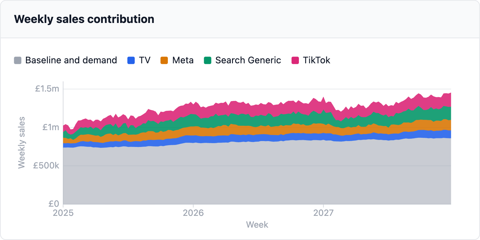
Now that we have a suitable data generating process, we can start by assessing the problem. When we use our generated data to build an MMM, what is the variance and bias, and how identifiable are adstock and saturation?

2. Three separate ways your model can mislead you

Now let’s move on to assessing the problem. There are three areas we are going to focus on:

• Variance. If you refit your MMM on a slightly different version of the same history, how far would its answer move?

• Bias. Across all those refits, does the average answer land on the truth, or is it consistently off to one side?

• Identifiability. Can the model recover each channel’s adstock and saturation?

Problem 1: Variance

We simulate 50 sales series from the data generating process. Each one keeps the spend, the response and demand fixed and only redraws the noise, so each is a version of the same three years that could equally have happened. We fit an MMM to each series, giving it the true demand and the true curve shapes, so the only thing that can make the estimates differ is noise meeting correlated spend. That is a best case: a real MMM has to estimate those too, so its estimates would move at least this much. We then compare each channel’s estimated incremental revenue on next year’s plan with the ground truth.

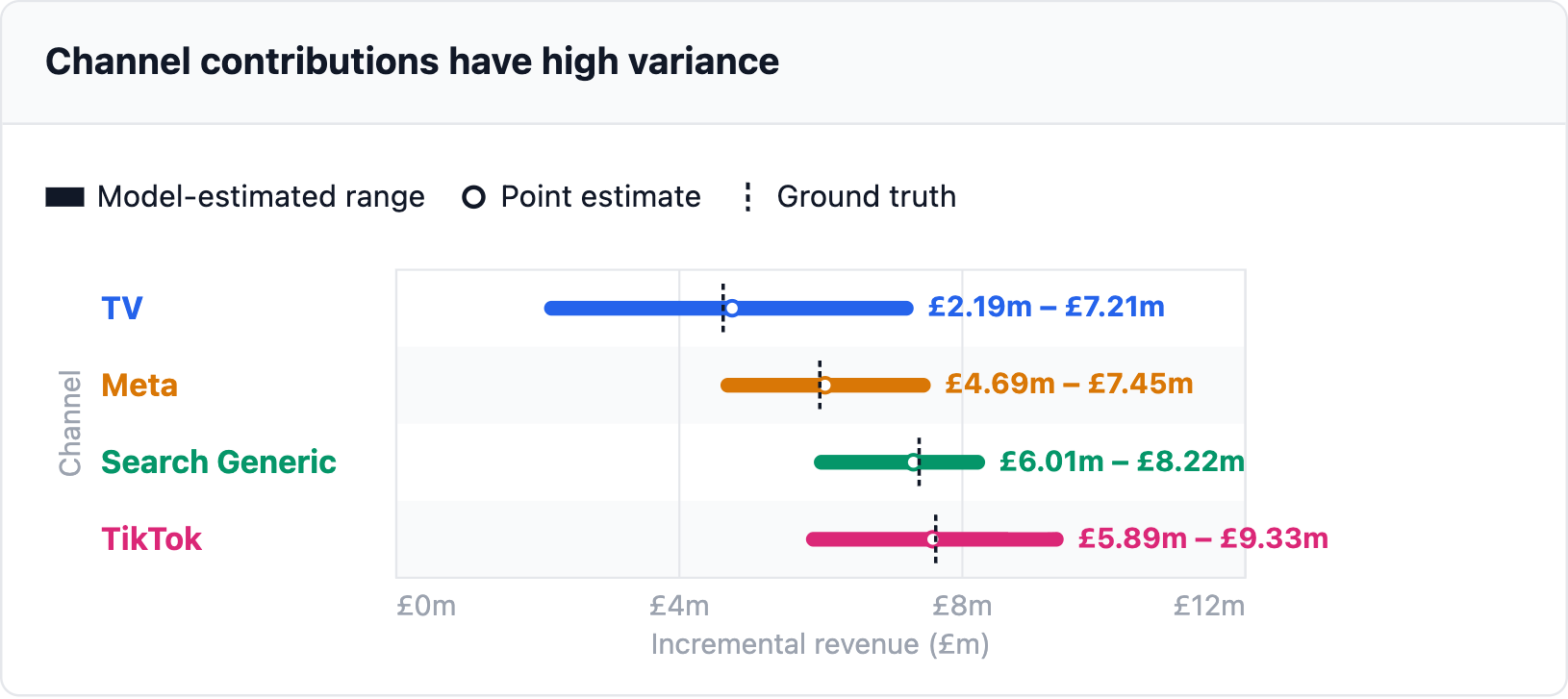
Look closely at how wide those ranges are. Any one of the four channels could have the highest incremental revenue. This isn’t bias: with correlated channels the regression still lands on the truth on average, as long as the model is specified correctly. The problem is that three years of weekly data contain very little independent movement per channel, so any single fit, including yours, could land anywhere in that range.

Problem 2: Bias

We fit the same way as for variance, with one change: the model gets the demand proxy instead of the true demand, just as a real MMM would. How large the bias is depends on the particular demand series and proxy we happen to draw, so a single draw could flatter or exaggerate it. We therefore draw 100 versions of demand and its proxy, run the 50 simulations on each, and compare the average estimate with the ground truth.

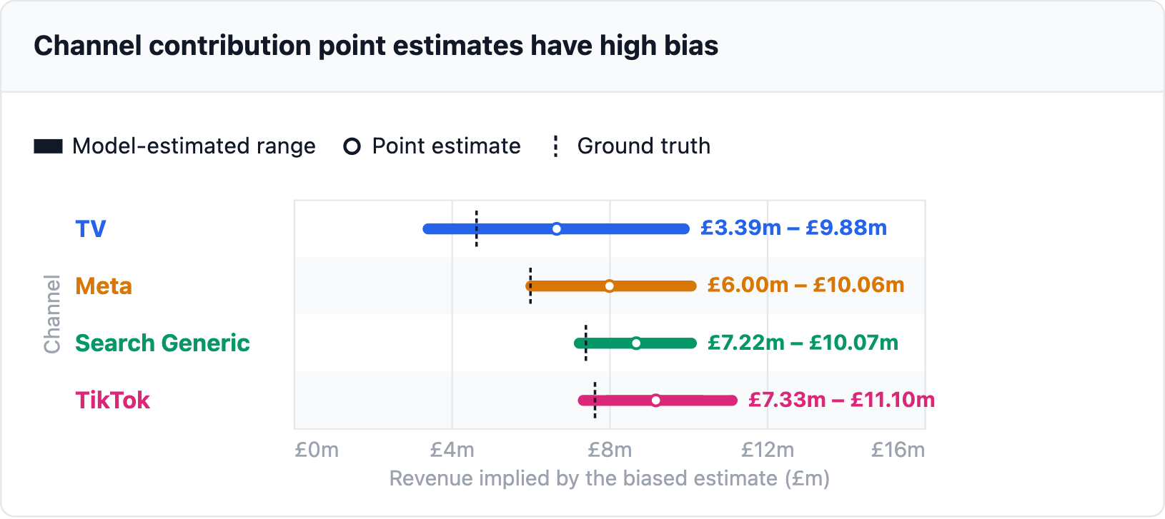
Pay attention to how the point estimates sit above the ground truth for every channel: TV by 44%, Meta by 33%, TikTok by 20% and Search Generic by 17%. This is driven by spend following demand. When demand lifts sales, spend is up too, and whatever the proxy misses gets credited to the channels. This is omitted variable bias, and unlike variance it doesn’t average out with more data. Refitting the same mis-specified model on more weeks just gets you a tighter estimate of the wrong number.

Problem 3: Identifiability

We simulate 50 sales series with fresh noise and give the model the true demand. We then take one channel at a time. The other channels keep their true saturation and adstock, and for the one being tested we try every combination of saturation exponent (0.20 to 1.00) and adstock decay (0.00 to 0.90) and keep the one that fits best. The spread of those best fits across the 50 series is the recovered range. This is a best case too: a real MMM has to estimate every channel’s shape at once.

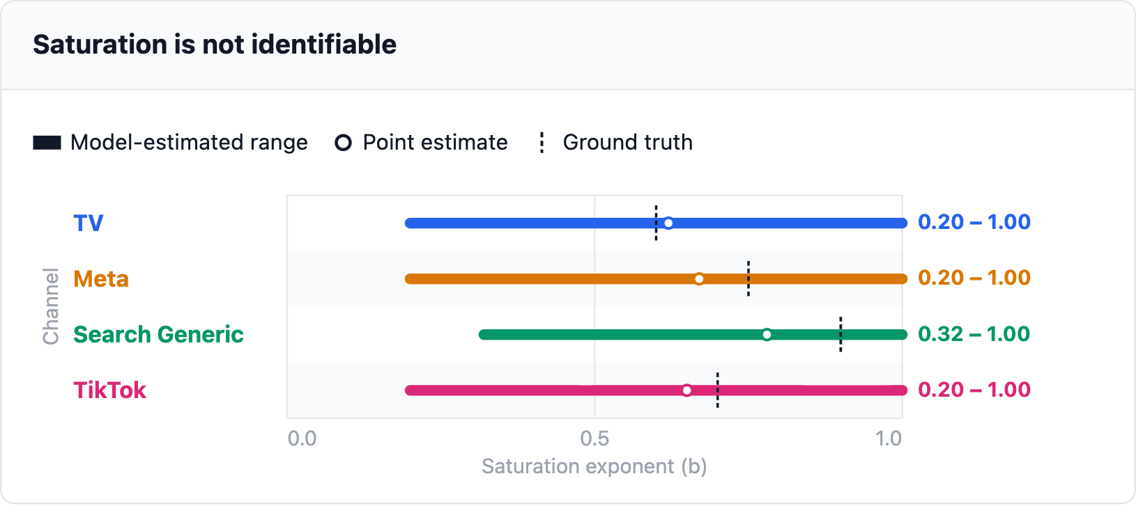
Saturation fares worst. For three of the four channels the range covers the whole 0.20 to 1.00 search. The model can’t tell TV’s bending curve (true 0.60) from a straight line, because seeing curvature needs a channel observed at clearly different spend levels while the others hold still. Here every channel rises and falls together, so a straight line and a curve fit the data about equally well.

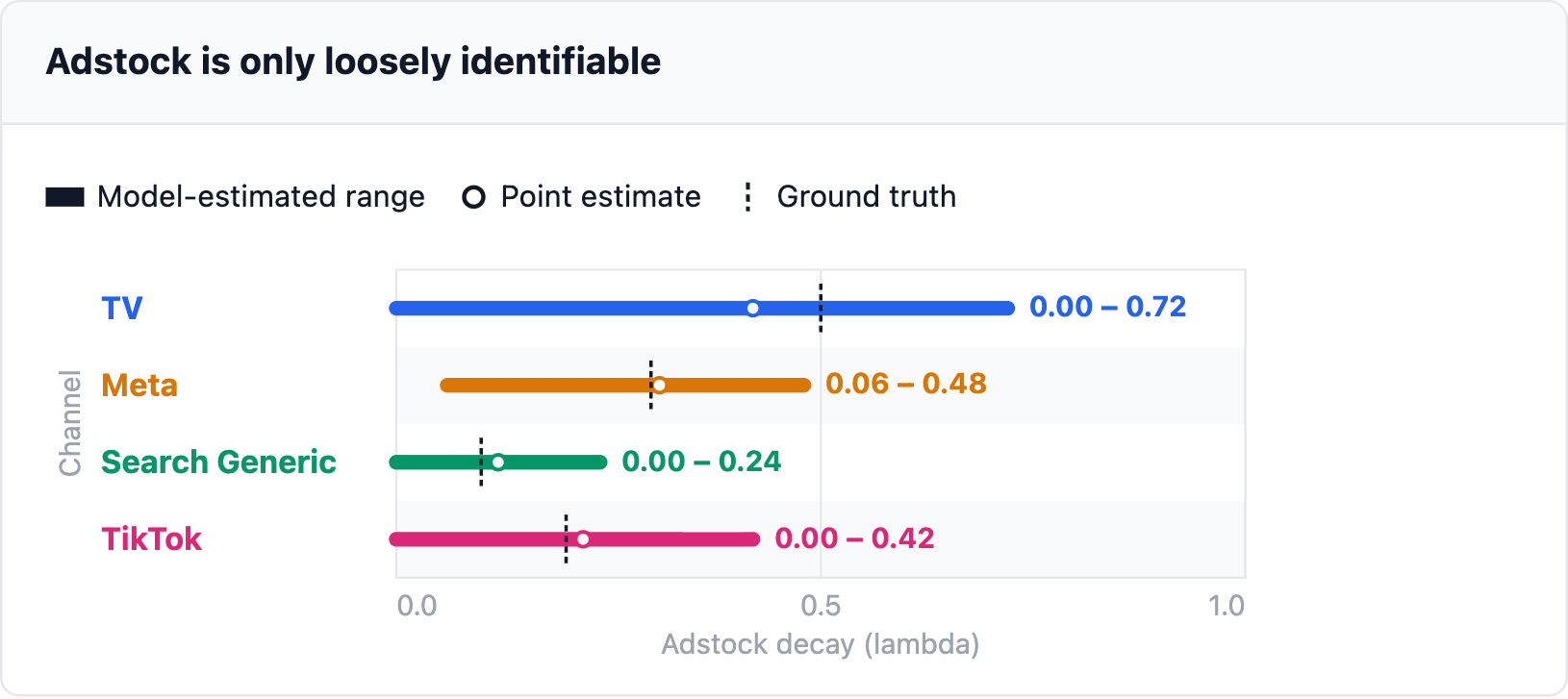
Adstock is better but still wide: every channel’s range reaches zero or close to it, so the model can’t rule out that ads stop working the week they run. TV’s true decay is 0.50, yet its range runs from 0.00 to 0.72.

Most teams respond to any one of these three problems by tweaking the model: different priors, different transformations, a different baseline or curvature specification. That rarely helps, because the model isn’t the problem. Channels that always moved together can’t be told apart by any estimation method, however sophisticated. In the next section we will dig a little deeper into the cause.

3. Your channels never move on their own

Here’s why the model is so unsure on all three counts. TV, Meta, Search Generic and TikTok budgets get set in the same planning cycle, so when one goes up, they usually all go up. In our data generating process every pair of channels has a correlation between 0.60 and 0.68.

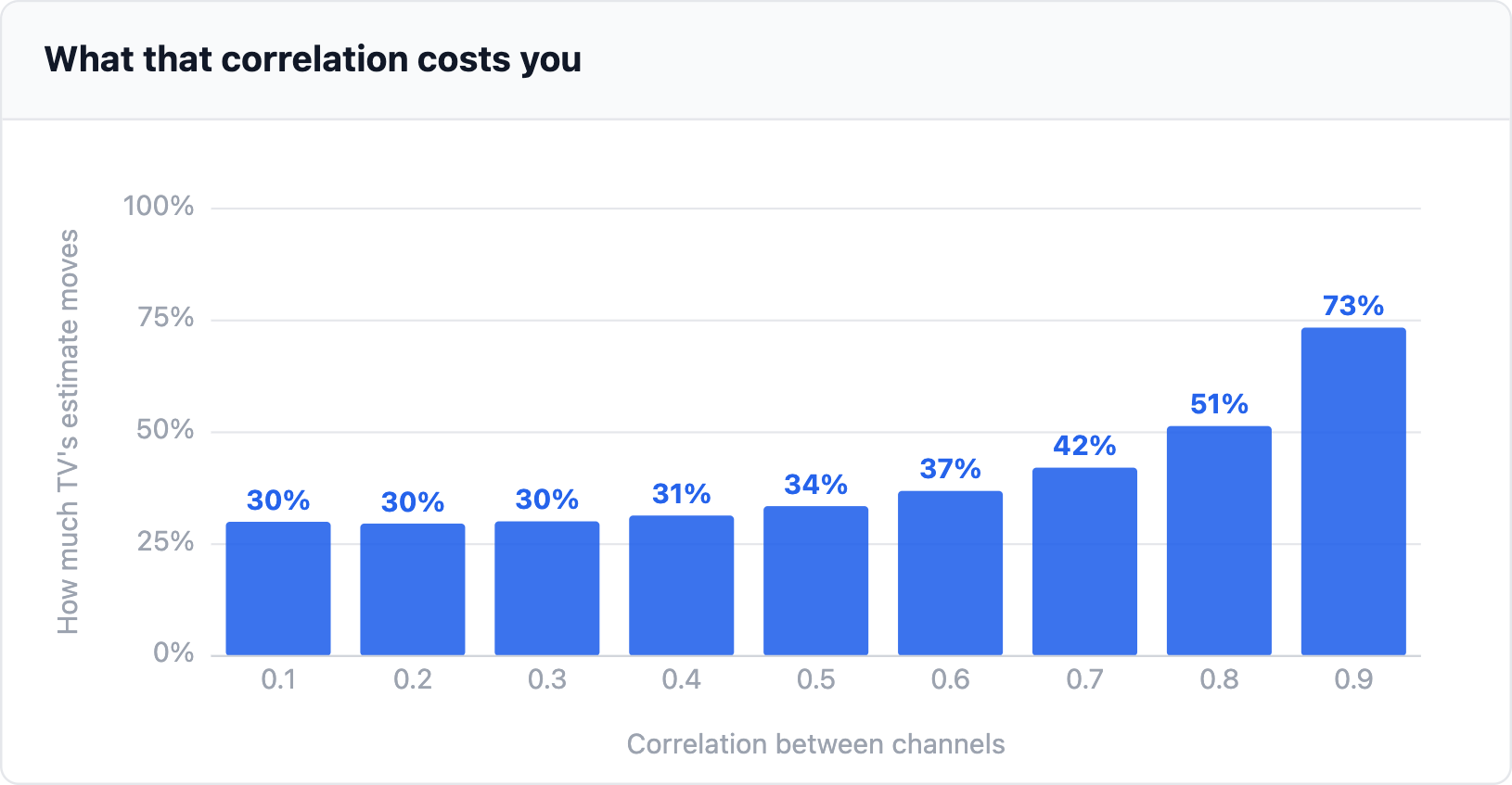
To see what that correlation costs, we rerun the variance measure from section 2 at every correlation from 0.1 to 0.9. Everything else is held fixed: the same budget and demand, the same response and the same week-to-week spread in spend. We track TV’s coefficient of variation: how much its estimated incremental revenue moves across refits, as a share of the estimate.

Even if the channels moved completely independently TV’s estimate would still move by about 30% of itself. That floor comes from sales noise and the amount of data rather than correlation. Correlation adds to it: 42% at our 0.7 and 73% at 0.9.

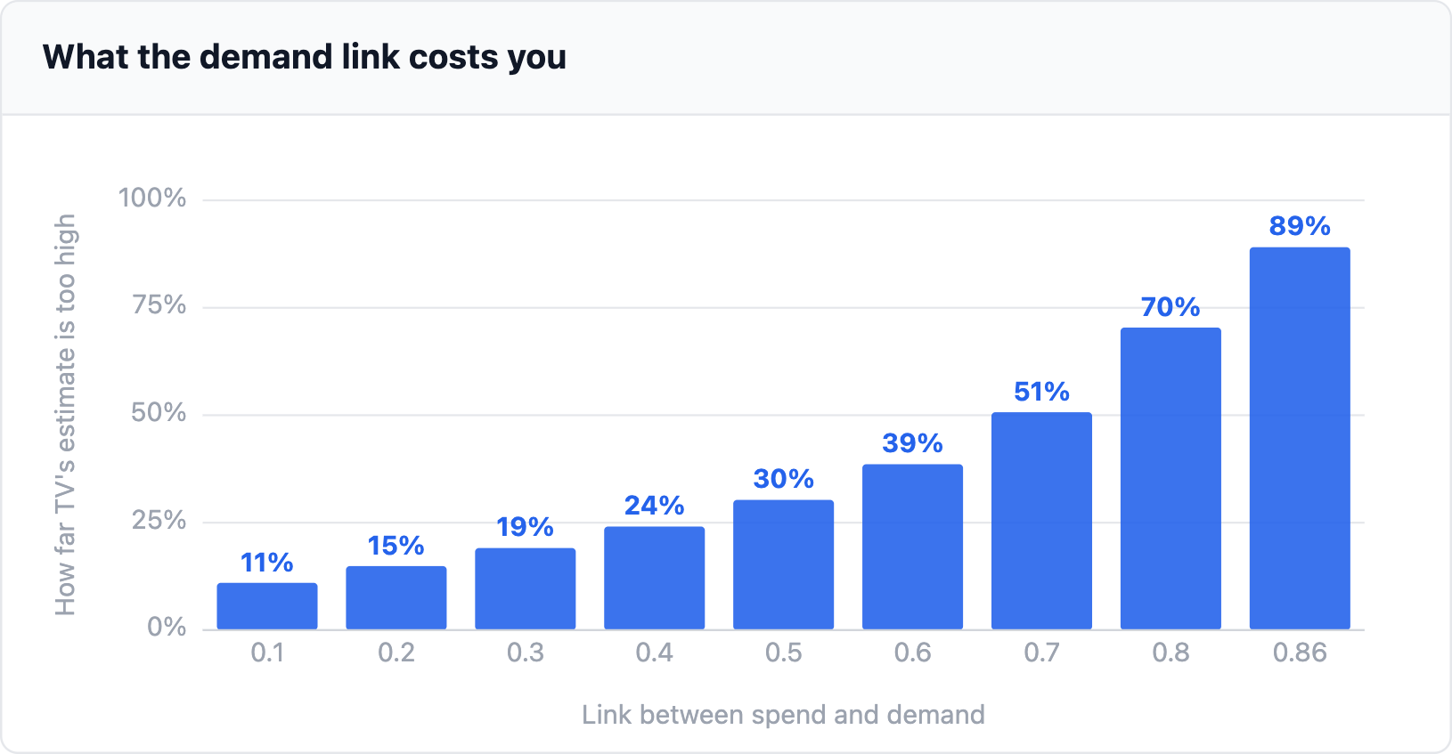
Bias works differently. It depends on how closely spend follows demand rather than how closely channels follow each other. So here we hold the channels at 0.7 and sweep the link between spend and demand instead (0.65 in our data generating process).

Even with a weak link of 0.1 TV’s estimate is 11% too high. At our 0.65 it is 44% too high and at 0.86 it is 89% too high. 0.86 is the strongest link possible when the channels sit at 0.7.

Adstock and saturation are a different kind of problem. Both need something from the spend itself. Adstock needs a change that is held for longer than the carryover lasts. Saturation needs spend at several clearly different levels. So there are three causes rather than one, and a fix has to supply a different kind of variation for each.

It isn’t that the model is badly built. It’s that the data it’s learning from was never designed to answer any of these three questions.

4. Same budget, a smarter phasing algorithm

You don’t need a bigger model, a bigger budget, or an AI agent bolted onto your MMM. You need spend that carries more information, and a phasing algorithm can supply it. That means each channel moving on its own, for reasons that have nothing to do with demand. It also means spend at several levels, each held for long enough to register.

The idea isn’t new. MMM vendors already say it: Recast tell clients to intentionally vary spend so the model becomes identifiable, and go-dark tests have been around for years. What has been missing is the how much. Which channel to move, by how far, and what you get back for it. This section goes into different phasing strategies, why we chose them and which works best.

What phasing has to do

Section 3 showed that each problem needs something different from the data. A phasing strategy has to supply it.

• Variance. Each channel has to move in weeks when the others don’t. Random moves, drawn separately for each channel, do this.

• Bias. The moves must have nothing to do with demand. A schedule drawn at random before the year starts can’t follow it.

• Adstock. A change has to be held for longer than the carryover lasts. Adstock smooths away a one-week blip, but a dark run or a month-long step survives it.

• Saturation. The channel needs spend well above its plan, held long enough to outlast adstock. Going dark doesn’t help here: zero spend gives zero response whatever the curve’s shape.

The strategies

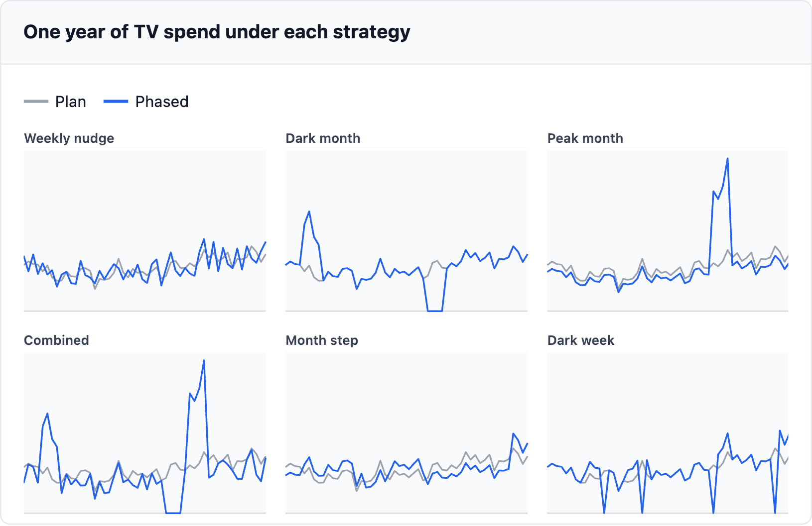
We test six strategies. The first three are building blocks, each aimed at one of the jobs above. The fourth runs all three together. The last two are lighter alternatives.

• Weekly nudge. Every week moves up or down by 20%. Ups and downs are balanced within the month, and the month is then rescaled to its planned total, which can lift the biggest week to 1.25 times plan. It is there for variance.

• Dark month. Once a year each channel goes dark for four weeks in a row. That budget moves into one other month. Channels take turns, so with up to 12 channels no two go dark in the same month. It is there for bias and adstock.

• Peak month. One month a year runs at 2.5 times plan. A small equal cut to the channel’s other months pays for it. Channels take turns, so with up to 12 channels no two peak in the same month. It is there for saturation.

• Combined. All three together: the dark month, the peak month, and the weekly nudge in every other month.

• Month step. Each whole month moves up or down by 20%. Every channel gets six up months and six down months. No two channels follow the same pattern.

• Dark week. One week a quarter goes dark, in a month picked at random. The rest of that month absorbs its budget.

Every strategy is drawn separately for each channel and keeps each channel’s annual budget. Weekly nudge and dark week also keep every month’s total. The other four move money between months.

We also tried two other weekly nudges: random sizes up to 20% and strict alternation between up and down. Neither improved on the fixed-size nudge, so they are left out.

Which works best

We run every strategy through the measures from section 2 and compare it with the unphased plan. Each strategy is averaged over 15 random draws of its schedule, and bias over 100 draws of demand.

The six strategies on this scenario

How to read the columns. Lower is better in every one:

• Variance: the coefficient of variation, averaged over the four channels.

• Bias: the mean absolute % gap from the truth, averaged over the four channels.

• Saturation and adstock: the average width of each channel’s range from section 2.

• Cost: the share of the revenue each channel drives in the plan year that is given up, averaged over the four channels.

• Peak: the biggest single week as a multiple of its plan.

Each figure is an average over many simulated runs, so it would move a little if we ran them again. Treat small gaps between strategies as ties.

Combined is best on all four diagnostics. Variance falls from 0.23 to 0.07 and bias from 28.8% to 15.3%. The saturation range more than halves from 0.77 to 0.31 and the adstock range falls from 0.45 to 0.18.

It also costs the most. Dark month is the closest alternative: it gets 92% of Combined’s variance gain and 71% of its bias gain for about half the cost (1.82% against 3.42%). What it can’t do is pin down saturation as well, where its range is 0.40 against Combined’s 0.31. Weekly nudge is the weakest: Month step beats it on variance and bias and is level on the rest, at the same cost.

Accuracy does not come for free. We think Combined’s extra accuracy is worth its cost, so it is the strategy we carry forward. If that cost is too high for you, Dark month is the place to start.

What it costs

• Revenue given up. Returns diminish as spend rises, so budget moved from a quiet week into a busy one earns less than it did. The cost follows how far spend is pushed up the curve, where each extra pound earns least. That is also what pins saturation down.

• Platform learning phases. Ad platforms can re-enter a learning phase after a large budget change and deliver worse while they do. We don’t model this. It is why the weekly nudges are capped at 20%. Dark months and peak months are much bigger moves, which is why the peak column matters.

Keep in mind that in our data generating process demand adds to sales and doesn’t change how well media works. If your media works harder when demand is high, moving spend out of busy weeks costs more than we show.

5. What the phasing algorithm buys you, and what it costs

From here on we focus on Combined, the best of the six strategies on this scenario.

The phased plan

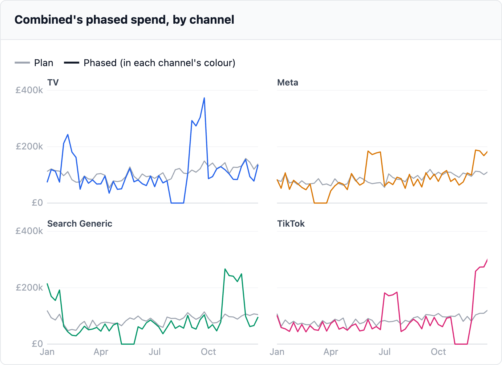
Each channel gets four dark weeks and two months well above plan: the one that takes the dark weeks’ budget and the peak month. No two channels go dark in the same month. In every other month each week moves up or down by 20%. Each channel’s annual budget is unchanged.

Correlation

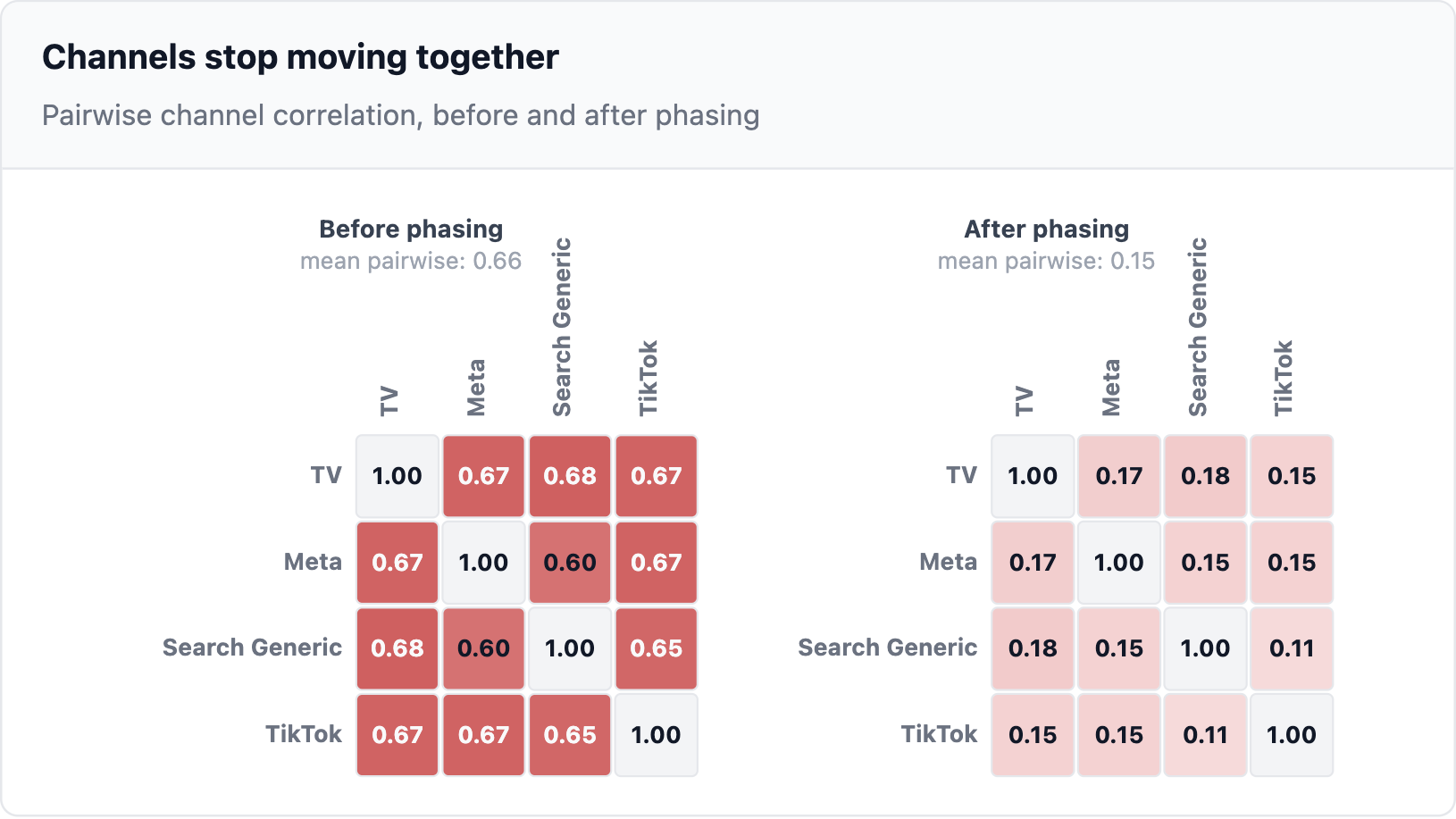
Before phasing every pair of channels moves together at between 0.60 and 0.68. After, every pair falls to between 0.11 (Search Generic/TikTok) and 0.18 (TV/Search Generic). Mean pairwise correlation falls from 0.66 to 0.15. Same channels and the same annual budget. Only the timing changed.

Impact 1: Variance

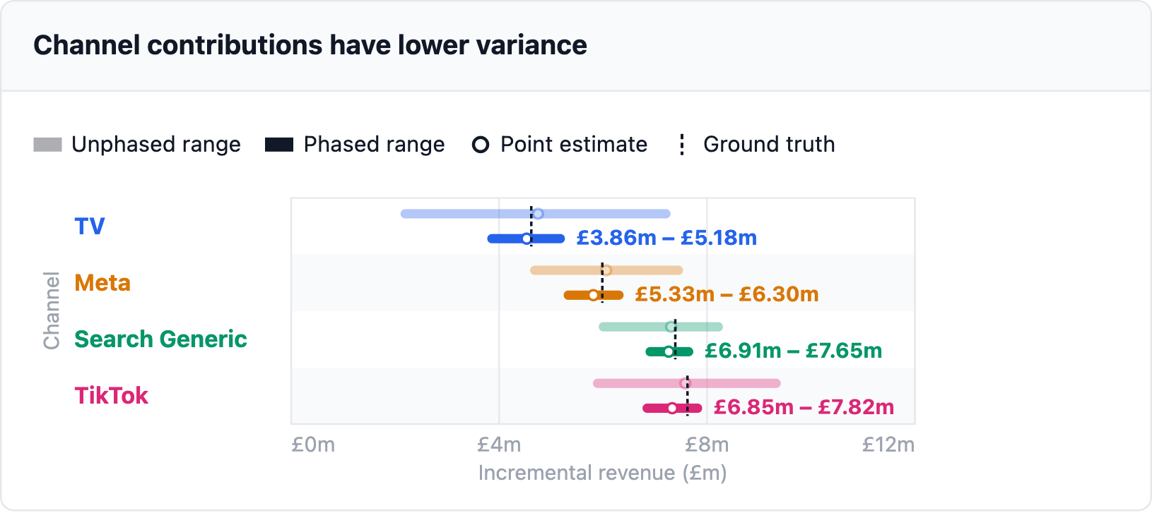
The range narrows for every channel: by 65% for Meta up to 74% for TV. The point estimate barely moves because variance is about the spread, not the centre.

Impact 2: Bias

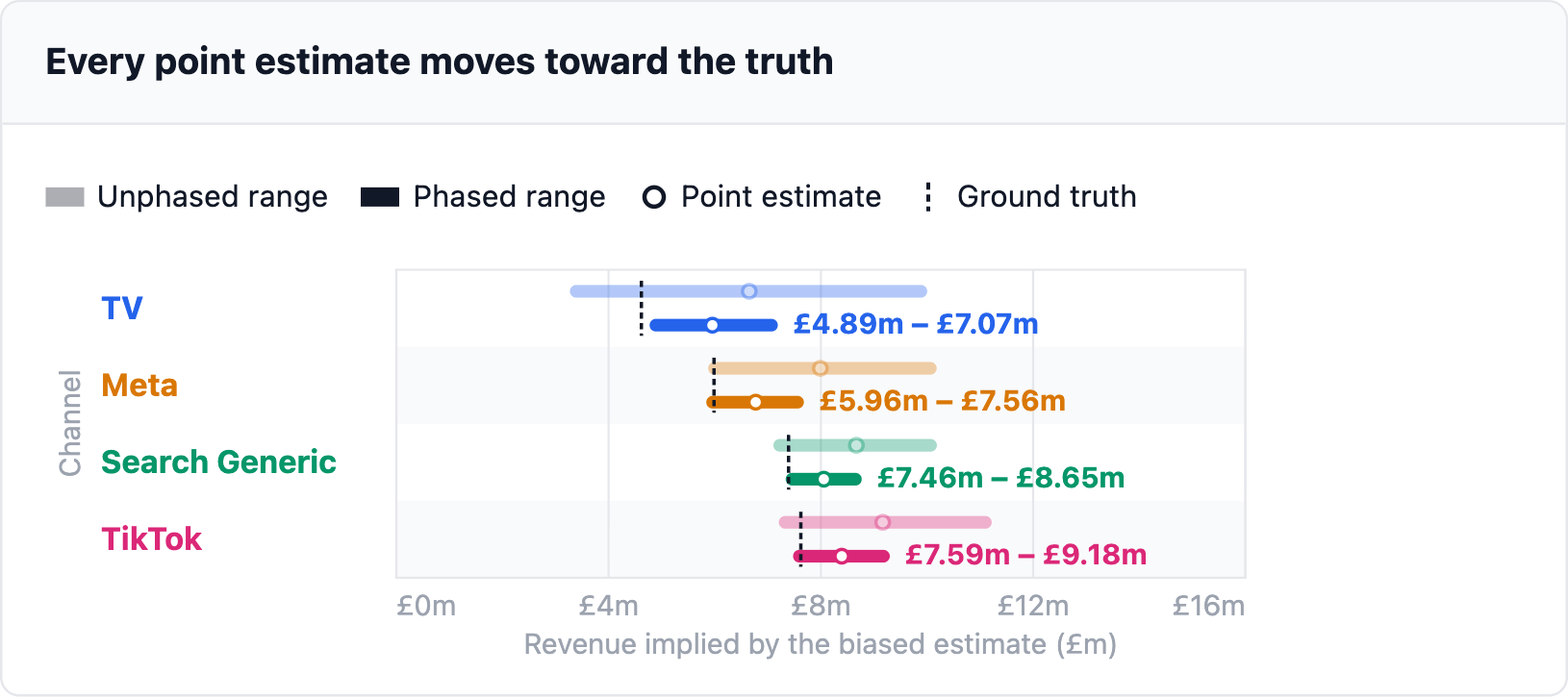
All four point estimates move toward the ground truth. TV’s bias falls from 44.0% to 29.0%, Meta’s from 33.5% to 13.1%, TikTok’s from 20.2% to 10.1% and Search Generic’s from 17.3% to 9.0%.

Impact 3: Identifiability

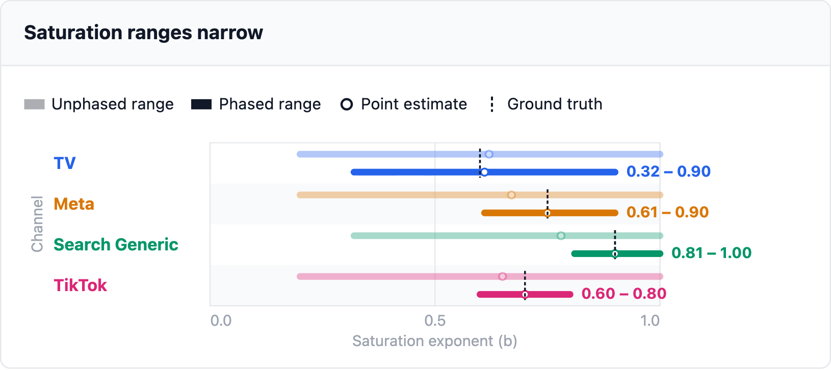
On saturation TV, Meta and TikTok no longer cover the whole 0.20 to 1.00 search. TV narrows the least: its range still runs from 0.32 to 0.90.

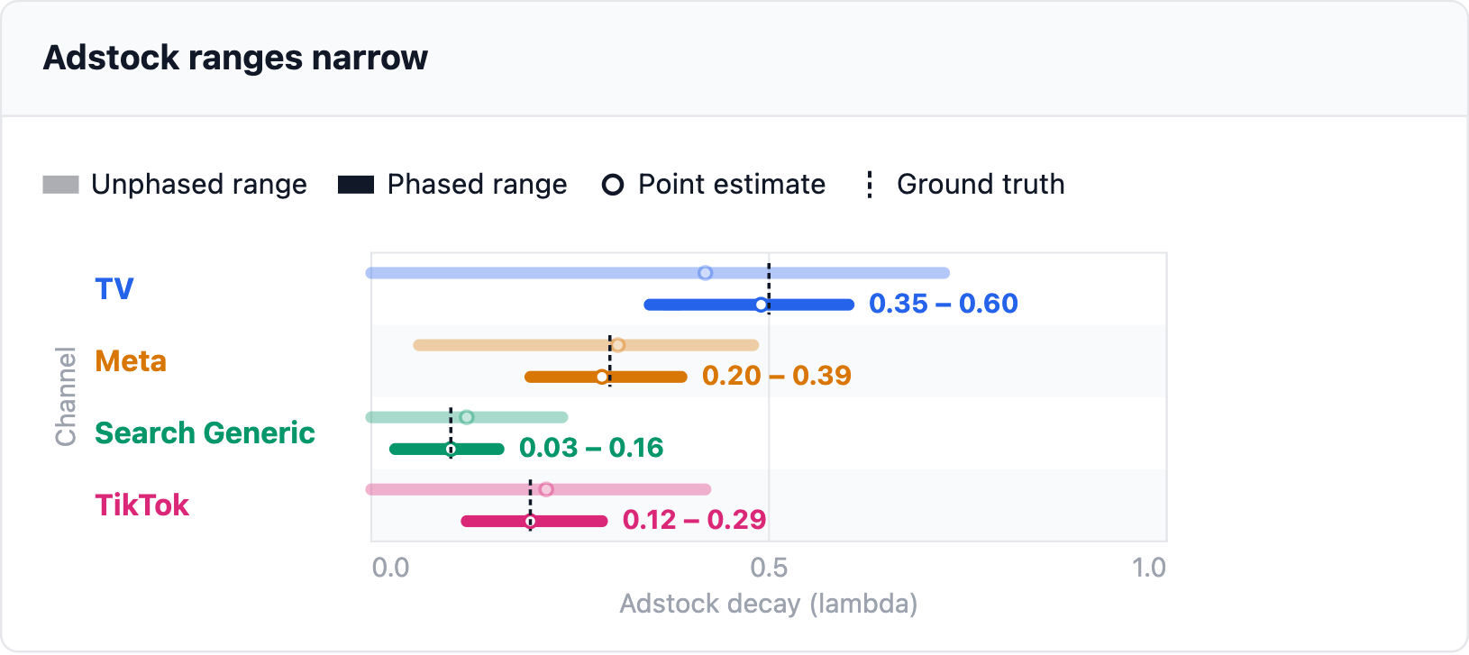
On adstock every range tightens, and TV and TikTok no longer reach down to zero. Search Generic was already tight and narrows a little, from 0.00–0.24 to 0.03–0.16.

How the benefit builds

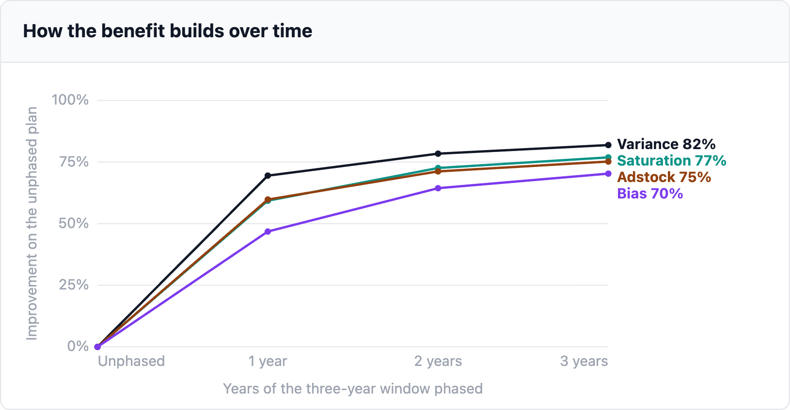
Everything above is after one year of phasing. The model is fitted on three years and only the last of them is phased. If the phasing keeps running the gains keep coming as more of the three-year window is phased.

Most of the gain lands in the first year. Year one delivers 85% of the three-year improvement in variance, 77% for saturation and 80% for adstock. Bias improves the slowest: 47% better after one year and 70% after three. The lines flatten by year three.

What it costs

Combined gives up 3.42% of the revenue the four channels drive in the plan year, the most of the six strategies. That is about £0.9m of £25.6m, or 1.5% of total sales. The annual plan stays at £19.0m and no extra spend is needed. Only the timing changes.

The cost depends on the saturation curves, which section 2 showed are hard to pin down. Keeping the same schedule and moving every channel’s exponent across that range, the cost runs from 0.3% when the curves are straight lines to 5.3% at an exponent of 0.4.

6. Does it scale to all of my channels?

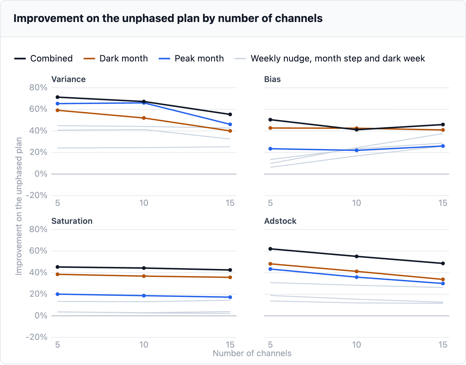
Everything so far uses four channels. Most MMMs have more than that, so in this section we test whether the phasing algorithm still works at 5, 10 and 15 channels.

We keep the data generating process from section 1 and only change the number of channels. Each added channel copies one of the four from section 1, and every pair still has a correlation of 0.7. The noise is held at its four-channel size. Because results at 10 and 15 channels vary from one simulated dataset to the next, every point is averaged over four of them.

The variance and adstock gains shrink as channels are added but hold up. At 15 channels Combined still cuts variance by more than half and bias by nearly half, and its saturation gain barely moves. Every strategy stays ahead of the unphased plan on every measure. The likely reason for the shrinkage is that the same three years of data are spread across more channels.

7. One pipeline, three steps

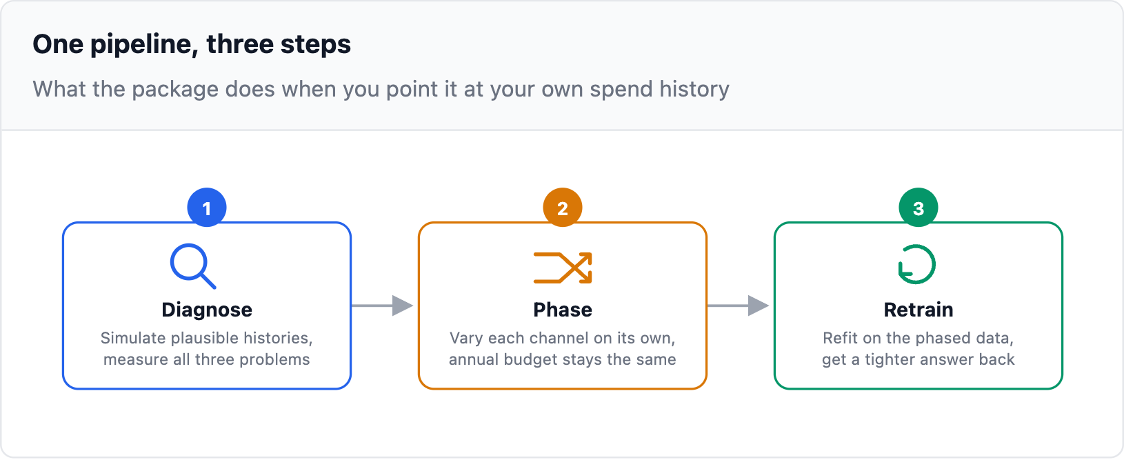
All of this runs through how_wrong_is_your_mmm, a free, open-source Python package. Point it at your own spend history and it runs the same three steps on your numbers, not a hypothetical example.

Step 1: Diagnose

You supply your weekly spend history and plan by channel. You also supply values from your MMM: each channel’s marginal return, saturation and adstock, plus the baseline, the noise and how closely spend follows demand. The package simulates many plausible versions of that history and refits an MMM on each one. It measures variance, bias and how identifiable adstock and saturation are. What comes back is a range per channel on each measure.

Step 2: Phase

It runs the six strategies from section 4, scores each one on the same measures and picks the one that does best. You get a week-by-week spend schedule for the plan year and what it costs in revenue. Each channel keeps its annual budget. Stronger settings can be pinned, and individual channels can be capped or left untouched.

Step 3: Retrain

You run that schedule, then refit your MMM on the data it produces. Because the channels no longer move together, the model can finally tell them apart, and the ranges come back narrower. Same budget, same annual total, a sharper answer.

Want to see what your team would actually get? See a full example report →

8. Frequently asked questions

Doesn’t this need me to already know my marginal return?

You supply a plausible estimate, not a proven one. The package uses it as the ground truth to measure against: it simulates revenue from that assumption, refits the model across many plausible versions of your history, and reports how far the answer moves. That spread tells you how reliable your model is, not whether your assumed number was right.

Why not just run a geo-lift test instead?

If you can run them, you should. Geo-experiments are the gold standard for a single channel. They take planning: you need regions you can hold out, and each test takes weeks or months to read. Testing several channels at once is possible with multi-cell designs, but it needs more regions and more budget. They aren’t immune to noise either: one simulation study by Recast found Meta’s GeoLift missed around 90% of real effects in its set-up. Phasing is not a replacement. It improves the data your MMM sees for every channel at once, and an experiment can then calibrate the channels that matter most.

Doesn’t a Bayesian model already fix this?

Not on its own. Priors are genuinely useful, and Google’s own Bayesian MMM paper shows why: they stabilise noisy estimates, and its flexible functional forms capture how spend decays and saturates over time. But priors can’t invent information that was never in the data. That paper says as much itself, noting that the optimal media mix it produces “has a large variance due to the variance of the parameter estimates”. If TV and Meta always moved together, no prior tells you which one actually drove sales.

But what about hierarchical models?

Genuinely useful, and worth doing if you can. Google’s own geo-level hierarchical paper shows that pooling across regions gives tighter intervals than national data alone. But your planning cycle is national, so TV and Search rise and fall together in every region: more rows, the same correlation inside each one. National TV and OOH are bought without a regional breakout, so any geo split there is an allocation rule rather than a measurement, and the paper is candid about what that costs: estimates “generally deteriorate as more media variables are imputed using the national level data”. Small regions are noisy on top of that. It helps, but it can’t manufacture variation your plan never had.

Won’t this put my channels into learning mode?

Possibly. Ad platforms can re-enter a learning phase after a large budget change, which is why the weekly nudges are capped at 20% (see section 4). Dark weeks and the budget they free up are bigger moves, so check the peak week before you commit. If a channel can’t take them, give it a lighter strategy rather than leaving it out. In our tests a channel left at its plan while the others were phased ended up with more bias than before, because it was the only one still following demand. It’s a compromise between data science and marketing, and each channel can be set separately.

What if a channel can’t take a dark month or a peak month?

Some can’t. TV is often booked upfront. Generic search can’t absorb 2.5 times its budget if the searches aren’t there. A dark month on one channel may dent another, such as TV driving search. We don’t model any of this, so give that channel a lighter strategy.

What about brand search and affiliates?

They are the hardest case for bias. With most channels you set a budget and demand only shapes it. With brand search and affiliates, demand sets the spend directly: you pay per click or per sale, so a good week for the business is automatically a big week for the channel. An MMM reads that as the channel driving the sales and gives it too much credit. This is endogeneity, and more data doesn’t fix it while spend keeps following sales. A weekly nudge doesn’t apply, because there is no fixed budget to nudge. A dark period does. Switching the channel off for a few weeks is a move in spend that demand didn’t cause, which is exactly what the model is missing.

What do I actually hand my media agency?

A weekly spend number per channel for the plan year. Each channel’s annual budget stays the same. The Combined strategy moves some budget between months, so the monthly totals change as well as the weekly split. Nothing about the buy itself changes, only when the money lands.

How do I phase a plan I haven’t finalised yet?

The budget phaser needs a starting weekly shape to work with, so build one the normal way: take your annual per-channel budget from your MMM and optimiser, and spread it across the year using whatever seasonality or demand pattern you’d use anyway. That first pass doesn’t need to be right; phasing is about to rework it regardless. Feed it in alongside your spend history, and the output is your real weekly booking plan, phased from day one instead of retrofitted onto something the agency’s already committed to.

9. It was never the model’s fault

Marketing budgets are planned together, follow demand and rarely leave their usual range. That leaves your MMM unsure in three separate ways. Its estimates move a long way from one refit to the next. They are biased by the demand it never saw. And it can’t tell the shape of your response curves. This article measures all three at once.

Budget phasing goes after the cause, which is spend that carries too little information. It changes when each channel spends and keeps each channel’s annual budget. On our scenario the Combined strategy cuts variance by 70% and bias by 47%. The saturation and adstock ranges narrow by 59% and 60%. It costs 3.42% of the revenue the channels drive, about £0.9m here. It holds from 5 to 15 channels, although the variance gain shrinks as channels are added. A Bayesian model doesn’t get around any of this: priors can’t create variation the data never had.

What comes next

This is a first version. Four things would make it more useful:

• Plug in your own MMM. Today the package refits its own simple MMM. The next step is to run the same checks with the model you already use, such as PyMC-Marketing, Meridian or Robyn. The inputs from section 1 could then come straight from its results.

• A strategy for each channel. Today one strategy is applied to every channel. But channels don’t start in the same place. One may already have low variance and bias and need no phasing. Another may need the full Combined treatment. The next step is to recommend the lightest strategy that fixes each channel, so you only pay the cost where it buys something.

• Keep phasing and re-plan. The schedule is set once for the year. A rolling version would re-plan each quarter from what was actually spent. It would aim the next quarter at the channels whose ranges are still widest.

• Optimise benefit against cost. Today the strategy is picked on variance, bias and identifiability, and the cost is shown next to it. The next step is to put a £ value on better estimates: the extra revenue from a better budget allocation, minus the revenue phasing gives up. That gives each strategy a payback period.

The question isn’t whether to trust your MMM. It’s whether your data gave it a fair chance, on variance, on bias, and on identifiability. Budget phasing is how you give it one, and this article shows what that costs as well as what it buys.

Want to find out how wrong your MMM is? Try the package →

···

Ryan O’Sullivan is a lead data scientist with over 16 years’ experience in causal inference and marketing mix modelling. Follow him on LinkedIn for more on marketing measurement.