Reparameterization Tricks: Variance Reduction by Smarter Gradients

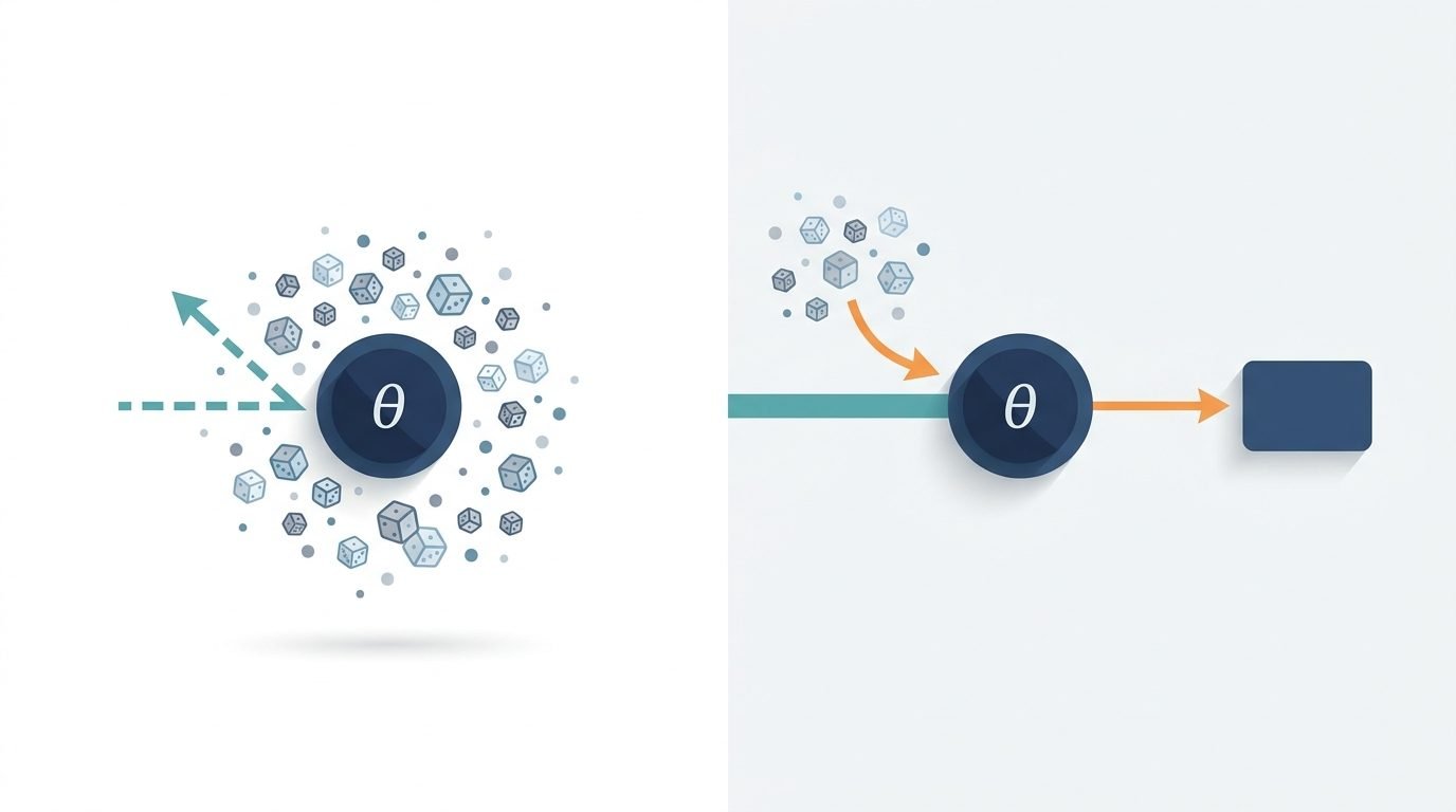
The reparameterization trick is what makes Variational Autoencoders (VAEs) trainable with standard stochastic gradient descent. It works by moving randomness outside the computation graph and turns an awkward gradient of an expectation into an ordinary chain-rule derivative.

A VAE is a generative model. An encoder maps input data xto a distribution over a latent variable z, while a decoder maps a sampled z back to a reconstruction of x. What makes it trainable is its objective, the ELBO (Evidence Lower Bound) i.e., a tractable stand-in for the true (intractable) data likelihood, made up of a reconstruction term and a term that regularizes the latent distribution toward a simple prior. To train a VAE involves maximizing this ELBO using gradient descent, and in order to do that the gradient of an expectation must be computed; more precisely, the gradient of the expected reconstruction quality with respect to randomly sampled latent variables z must be computed.

It’s genuinely awkward to make that distinction and the issue is not unique to VAEs. The same structure shows up in the expected return in policy-gradient RL, and in variational inference more generally. In every case we’re optimizing L(θ) = E[f(z)] where z is itself sampled from a distribution that depends on θ — so the thing we’re differentiating is defined by the distribution we’re differentiating with respect to. That circularity is where a lot of the pain in stochastic optimization comes from, and it’s exactly what the reparameterization trick was built to sidestep.

This article walks through that problem, the two main families of gradient estimators used to solve it, and why the “pathwise” gradients obtained through reparameterization tend to have dramatically lower variance than the alternative.

Why low-variance gradients matter in practice

A lower-variance gradient estimator is not just a theoretical nicety. In practice, it directly translates to:

1. More stable training curves — fewer wild swings in the loss.

2. Faster convergence — can take larger effective steps with less noise.

3. Better final models — the optimizer spends less time fighting gradient noise and more time fitting the data.

This is especially critical for complex models like VAEs, Bayesian neural networks, and continuous-control Reinforcement Learning agents, where the training signal can otherwise be too noisy to be useful.

The problem: Gradients of expectations — why sampling breaks backprop

Suppose we want to optimize

with respect to θ. If θ only appeared inside f, this would be a standard backprop problem. The complication is that θ parameterizes the distribution that z is drawn from — the sampling process itself depends on θ — so we can’t just push the gradient through a fixed computation graph. Monte Carlo estimates of L(θ) are easy (draw samples, average f(z)), but Monte Carlo estimates of ∇θ L(θ) are not automatic, because differentiating through a sampling operation isn’t well defined.

There are two general ways out of this: the score function estimator (REINFORCE) and the pathwise / reparameterization estimator. Both are unbiased. They differ enormously in variance.

The score function estimator (REINFORCE): flexible but high variance

The classic trick here is the log-derivative identity:

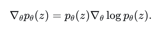
Substituting this into the gradient of the expectation gives

which is now an expectation again, so it can be estimated by sampling z ~ p_θ and averaging f(z)·∇θ log p_θ(z). This is the estimator behind REINFORCE in policy-gradient reinforcement learning, and it’s genuinely versatile. It works for discrete zand it doesn’t require f to be differentiable at all. Only p_θ needs a tractable, differentiable log-density.

The cost of that generality is variance. The estimator only ever sees the scalar value f(z). It has no information about how f changes as z changes. When f(z) is roughly the same for most sampled z but the score ∇θ log p_θ(z) fluctuates a lot (which it does, especially in high dimensions or with peaked distributions), the product f(z)·score becomes a noisy quantity with high variance, and that noise shows up directly in the gradient estimate. This is why REINFORCE-style estimators almost always need variance-reduction machinery bolted on — baselines, control variates, advantage normalization; to be usable in practice.

The reparameterization trick: pathwise gradients made differentiable

The alternative is to change how we generate z. Instead of sampling z directly from p_θ, we express z as a deterministic, differentiable function of θ and an auxiliary noise variable ε whose distribution does not depend on θ:

The canonical example is the Gaussian: instead of sampling z ~ N(μ, σ²) directly, sample ε ~ N(0, 1) and set z = μ + σ·ε. All the randomness now lives in ε, which is fixed and independent of θ. θ only enters through a deterministic transformation.

With that reformulation, the expectation becomes

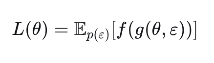
and because the distribution we’re integrating over no longer depends on θ, we can push the gradient straight inside:

This is the pathwise derivative: for each sampled ε, we differentiate f through the deterministic path z = g(θ, ε) using the ordinary chain rule, exactly as if we were backpropagating through any other layer in a neural network. In fact, once z is reparameterized this way, sampling becomes just another differentiable operation in the computation graph, and standard autodiff handles the rest.

Why reparameterization reduces gradient variance

The intuitive reason pathwise gradients tend to be much lower variance is that they actually use local, first-order information about f i.e., the derivative f'(z); whereas the score-function estimator only ever uses the value f(z). Two samples that land close together in z-space will have similar pathwise gradient contributions (because f is locally smooth), but they can have wildly different score-function contributions, because the score ∇θ log p_θ(z) doesn’t know anything about f and can swing sharply even between nearby points. The pathwise estimator effectively differentiates the reward surface directly. The score-function estimator has to infer sensitivity to θ indirectly, by looking at how much more or less likely a given sample becomes. This is a much noisier signal. This comparison is formalized nicely in Mohamed et al.’s survey on Monte Carlo gradient estimation, which frames both estimators within a common framework and derives conditions under which each has lower variance.

A numerical example: score function vs reparameterization

Take the toy problem L(θ) = E[z²], z ~ N(θ, 1), for which the true gradient is simply 2θ. Estimating this gradient two ways: score function vs. reparameterization, with the same number of samples per estimate:

import numpy as npimport matplotlib.pyplot as pltnp.random.seed(0)theta = 1.5sigma = 1.0true_grad = 2 * thetadef score_function_grad(n):    z = np.random.normal(theta, sigma, size=n)    f = z**2    score = (z - theta) / sigma**2       # d/dtheta log N(z; theta, sigma^2)    return (f * score).mean()def reparam_grad(n):    eps = np.random.normal(0, 1, size=n)    z = theta + sigma * eps    return (2 * z).mean()                # df/dtheta via chain rule, dz/dtheta = 1n = 20sf = np.array([score_function_grad(n) for _ in range(20000)])rp = np.array([reparam_grad(n) for _ in range(20000)])print("true grad:", true_grad)print("score-function  mean/var:", sf.mean(), sf.var())print("reparameterized mean/var:", rp.mean(), rp.var())print("variance ratio (SF / reparam):", sf.var() / rp.var())plt.hist(sf, bins=50, alpha=0.5, label="Score function")plt.hist(rp, bins=50, alpha=0.5, label="Reparameterization")plt.axvline(true_grad, color="k", linestyle="--", label="True gradient")plt.legend()plt.xlabel("Gradient estimate")plt.ylabel("Frequency")plt.title("Distribution of gradient estimates (n = 20)")plt.show()

Running this gives both estimators converging to the correct gradient (≈3.0) on average, but with

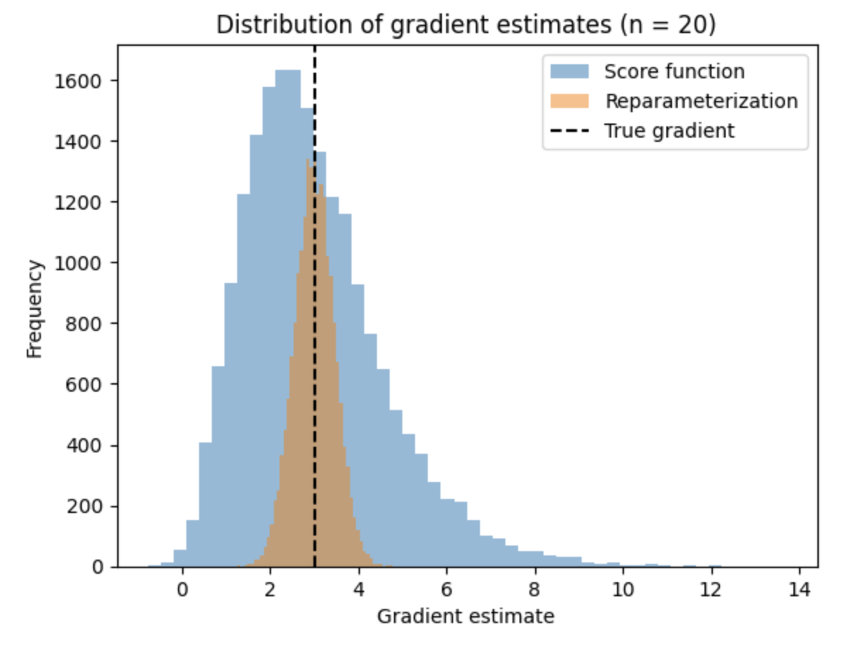
Histogram comparing the distribution of score-function and reparameterized gradient estimates; the reparameterized estimates cluster tightly around the true gradient.

Roughly a 13x reduction in variance from reparameterization alone, on a problem this simple. In higher-dimensional, more peaked posteriors, the regime VAEs and variational inference actually operate in, the gap tends to widen further, which is a big part of why reparameterized ELBO estimators made scalable variational inference practical in the first place.

When can we use the reparameterization trick?

Reparameterization isn’t free. It requires a differentiable sampling path, which not every distribution has in closed form.

• Location-scale families (Gaussian, Logistic, Laplace, uniform) reparameterize trivially, as above.

• Distributions with a tractable inverse CDF can be reparameterized via inverse-transform sampling: draw u ~ Uniform(0,1) and set z = F_θ⁻¹(u).

• More complex continuous distributions (Gamma, Beta, Dirichlet, von Mises) don’t have a simple location-scale form, but can still be handled through implicit reparameterization gradients, which differentiate through the CDF itself rather than requiring an explicit sampling path (Figurnov et al., 2018).

• Discrete random variables (categorical, Bernoulli) have no differentiable sampling path. Small changes in θ don’t change z continuously. The standard workaround is a continuous relaxation: the Gumbel-Softmax / Concrete distribution replaces the hard discrete sample with a temperature-controlled continuous approximation that is reparameterizable, trading a small amount of bias for a reparameterized low-variance gradient (Jang, Gu & Poole, 2016; Maddison, Mnih & Teh, 2016).

• Even within reparameterizable models, further variance reduction is possible. For instance, the “sticking the landing” trick removes a score-function term that leaks back into supposedly pathwise ELBO gradients as the approximate posterior converges to the true one (Roeder, Wu & Duvenaud, 2017).

Reparameterization in practice: VAEs, RL, and variational inference

• Variational autoencoders use reparameterization to get low-variance gradients of the ELBO with respect to the encoder parameters. This is essentially what made VAEs trainable with standard SGD (Kingma & Welling, 2013; Rezende, Mohamed & Wierstra, 2014).

• Policy-gradient reinforcement learning with continuous action spaces can use the reparameterized (“pathwise”) policy gradient instead of REINFORCE, which is one of the reasons algorithms like Soft Actor-Critic are comparatively sample-efficient.

• Variational inference more broadly (Bayesian deep learning, Bayesian neural networks, probabilistic programming) relies on reparameterized gradients to fit approximate posteriors via stochastic optimization instead of MCMC.

Score function vs pathwise estimator: summary

The reparameterization trick is not a different optimisation algorithm; rather, it is a change of variables that converts ‘differentiating through a sampling process’ into ‘differentiating through an ordinary deterministic function’, allowing the chain rule to carry out the task it is good at. Since such a transformation is possible whenever the underlying distribution allows it, it is almost always worth using as a replacement for a score-function estimator, simply because it provides the optimizer with a much cleaner gradient signal.

References

For all the articles I have referenced in this article, you can check these links.

1. Kingma, D. P., & Welling, M. (2013). Auto-Encoding Variational Bayes. arxiv.org/abs/1312.6114

2. Rezende, D. J., Mohamed, S., & Wierstra, D. (2014). Stochastic Backpropagation and Approximate Inference in Deep Generative Models. arxiv.org/abs/1401.4082

3. Mohamed, S., Rosca, M., Figurnov, M., & Mnih, A. (2020). Monte Carlo Gradient Estimation in Machine Learning. Journal of Machine Learning Research. jmlr.org/papers/v21/19-346.html

4. Figurnov, M., Mohamed, S., & Mnih, A. (2018). Implicit Reparameterization Gradients. arxiv.org/abs/1805.08498

5. Jang, E., Gu, S., & Poole, B. (2016). Categorical Reparameterization with Gumbel-Softmax. arxiv.org/abs/1611.01144

6. Maddison, C. J., Mnih, A., & Teh, Y. W. (2016). The Concrete Distribution: A Continuous Relaxation of Discrete Random Variables. arxiv.org/abs/1611.00712

7. Roeder, G., Wu, Y., & Duvenaud, D. (2017). Sticking the Landing: Simple, Lower-Variance Gradient Estimators for Variational Inference. arxiv.org/abs/1703.09194

8. Williams, R. J. (1992). Simple Statistical Gradient-Following Algorithms for Connectionist Reinforcement Learning. Machine Learning, 8, 229–256. (Original REINFORCE paper.) link.springer.com/article/10.1007/BF00992696