How to Make Linear Regression Survive Outliers

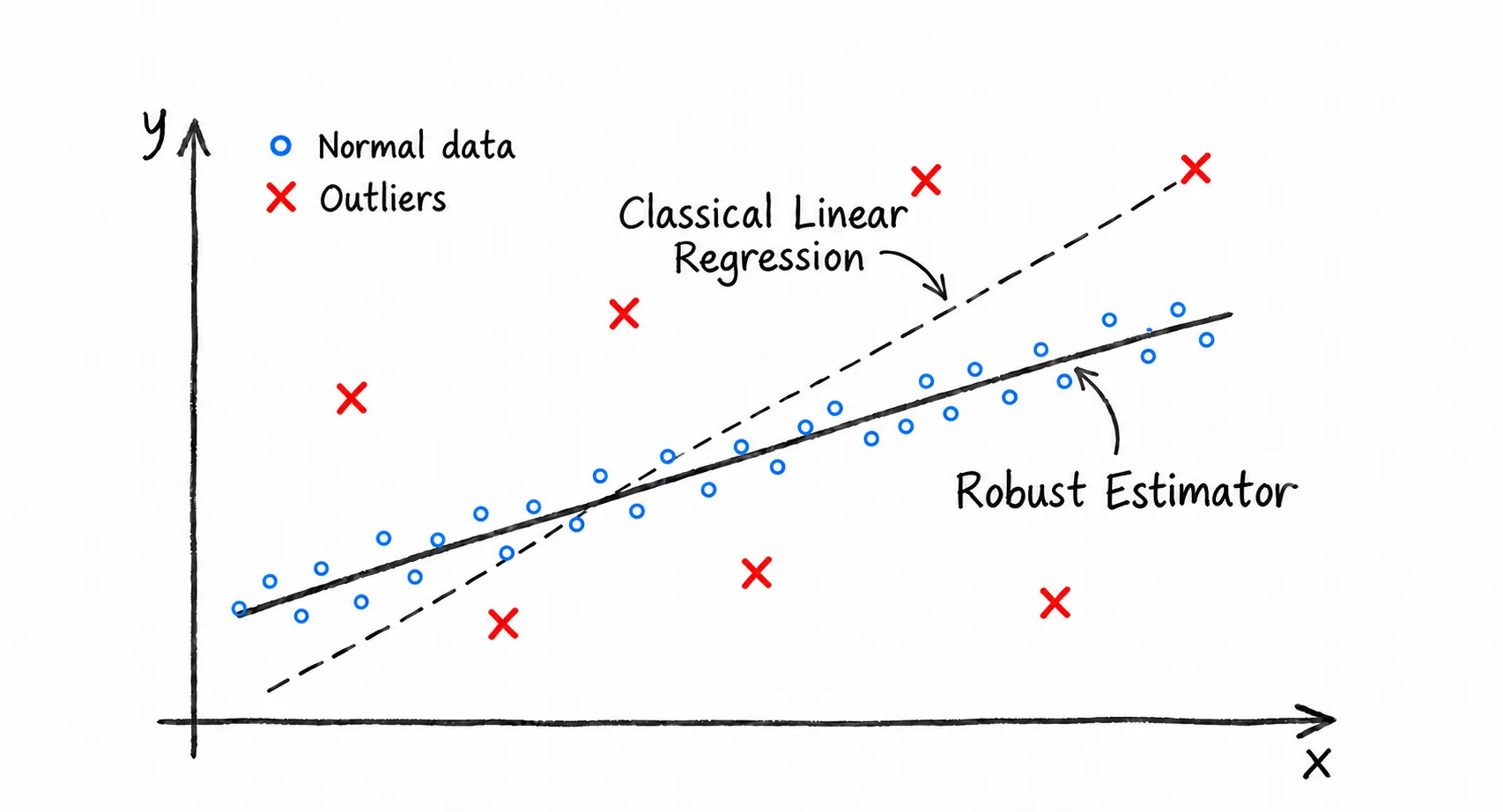
A simple model with a serious weakness

A straight line can look surprisingly convincing—until a few bad measurements pull it somewhere it should never have gone.

Linear regression is often one of the first predictive models practitioners learn—and one of the first they set aside when more sophisticated machine-learning methods become available. Yet linear models remain valuable when coefficients need a physical interpretation, predictions must run on a resource-constrained device, computational latency matters, or a simple benchmark is needed before introducing a higher-capacity model. They are also useful as local approximations: even a complex nonlinear relationship may behave approximately linearly over a sufficiently small region.

Its simplicity, however, comes with an important weakness:

Ordinary Least Squares treats every observation as trustworthy.

In real data, that assumption is easy to violate. A faulty sensor, communication error, calibration problem, or biased measurement can produce observations far from the relationship we actually want to estimate. Because Ordinary Least Squares (OLS) squares every residual, a few such observations can have a disproportionate effect. Robust estimators try to prevent those observations from dominating the fit.

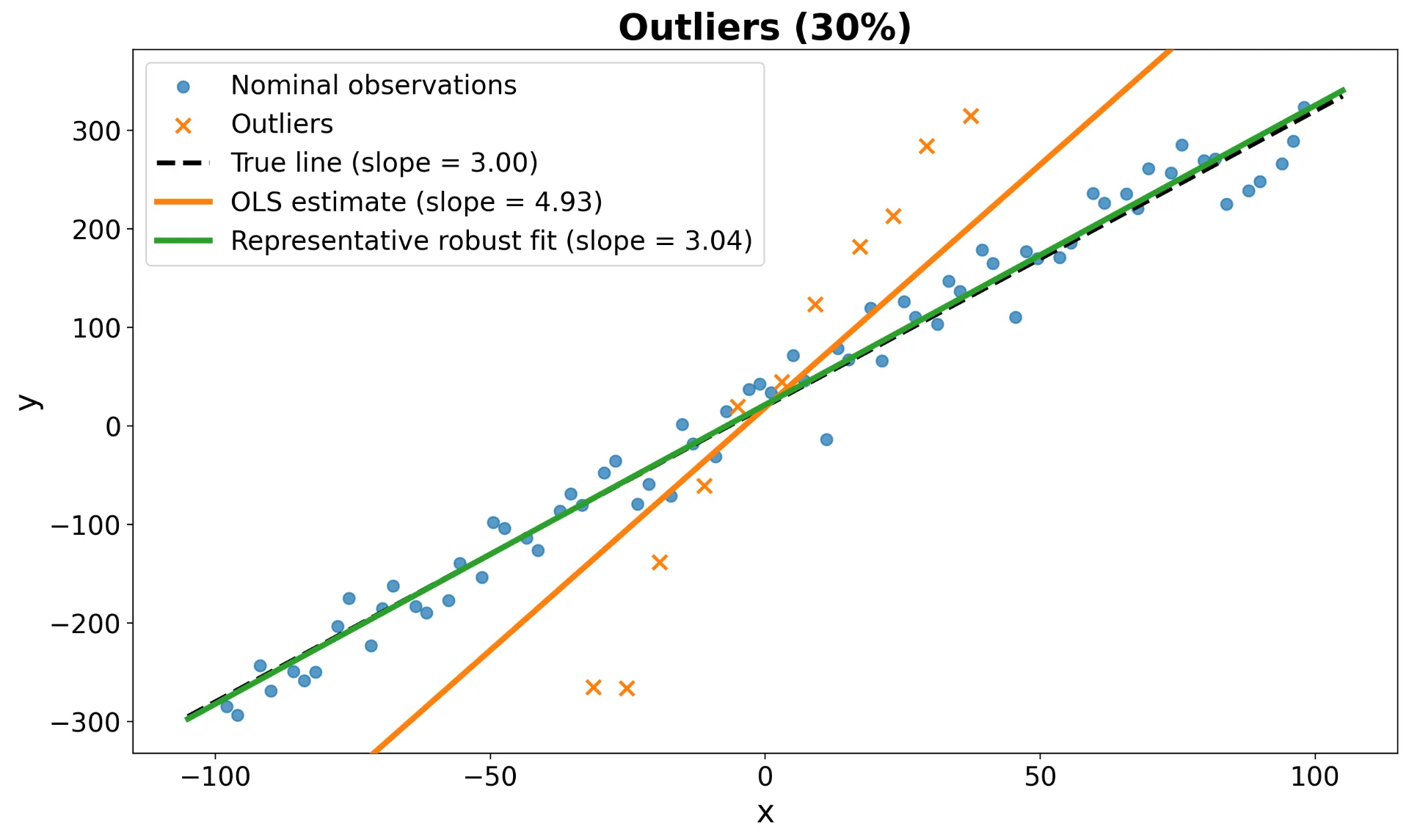
Figures 1 and 2 show how quickly the picture can change. With clean observations, OLS follows the nominal relationship closely. After 30% of the responses are replaced by outliers, the same estimator is pulled sharply away from it. A representative robust fit, however, stays much closer to the relationship supported by the nominal observations.

That leads to the practical question I want to explore in this article:

How do different robust estimators behave when we do not know the outlier statistics in advance—and when the contamination becomes progressively harder?

Knowing that a dataset contains outliers is only part of the problem. In practice, we rarely know their percentage, bias, variance, distribution, or structure beforehand. A method that works well for one convenient outlier model may behave very differently under another. The estimators here are therefore tested across several deliberately different forms of contamination.

This article compares OLS as the non-robust baseline (Legendre, 1805) with five robust estimators: Huber regression (Huber, 1964), Random Sample Consensus (RANSAC; Fischler and Bolles, 1981), Graduated Non-Convexity with the Geman–McClure loss (GNC-GM), Graduated Non-Convexity with the Truncated Least-Squares loss (GNC-TLS; Yang et al., 2020), and Adaptive Selective Outlier Rejecting (ASOR; Chughtai et al., 2024).

Huber regression and RANSAC are classical robust-estimation methods, whereas GNC-GM, GNC-TLS, and ASOR represent more recent approaches based on non-convex continuation and adaptive residual weighting. Their central algorithmic steps are implemented directly so that the weighting, rejection, sampling, stopping, and continuation mechanisms remain visible.

The estimators are evaluated using prediction error and runtime to capture both statistical accuracy and computational efficiency.

Disclosure. The author developed ASOR in the original study cited here. To ensure a transparent comparison, all estimators are evaluated on the same Monte Carlo realizations using fixed and documented settings.

Why squared loss can be dominated by a few observations

To see why a few bad measurements can have so much influence, consider the scalar linear model:

Here, $β₀$

For$N$independent observations, maximizing the likelihood with respect to $β$ is equivalent to minimizing the OLS objective:

where

When $boldsymbol{X}$ has full column rank, the familiar closed-form expression is:

A numerical least-squares solver is preferable to explicitly forming the inverse:

def fit_ols(x, y):    X = np.column_stack((np.ones_like(x), x))    return np.linalg.lstsq(X, y, rcond=None)[0]

The same squared-loss objective that makes OLS simple and efficient also creates its main weakness. The contribution of an observation grows quadratically with its residual magnitude:

Thus, a normalized residual of $100$ contributes as much to the OLS objective as $10000$ normalized residuals of $1$. A small number of severe outliers can therefore pull the fitted model away from the relationship supported by most observations, as demonstrated in Figure 2.

Practical note on missing values. Rows containing a missing predictor or response can be excluded before fitting:

valid = np.isfinite(X).all(axis=1) & np.isfinite(y)X = X[valid]y = y[valid]

This treatment is appropriate when missing values are limited and non-systematic. Outliers, however, are different. Missing observations can usually be identified before fitting, whereas outliers must be inferred from residuals that depend on the unknown regression model. Since the fitted model is itself influenced by the outliers, model estimation and outlier identification must be performed jointly.

Six estimators, one shared idea

Table 1. Robustness mechanisms and principal limitations of the six estimators.

A common way to achieve this joint treatment is to control the influence of each observation through a residual-dependent weight. Most methods in this comparison therefore repeatedly solve a weighted least-squares problem:

The sum runs over all $N$observations, and the normalized residual is:

Here, $w_i$

A shared weighted least-squares engine

Most estimators in this comparison repeatedly solve the same weighted least-squares problem. To keep their method-specific weighting, sampling, and continuation mechanisms visible, they use the following shared numerical solver:

def weighted_least_squares(x, y, weights=None):    X = np.column_stack((np.ones_like(x), x))    if weights is None:        weights = np.ones(len(y))    sqrt_w = np.sqrt(        np.asarray(weights, dtype=float)    )    Xw = X * sqrt_w[:, None]    yw = np.asarray(y, dtype=float) * sqrt_w    beta, _, rank, _ = np.linalg.lstsq(        Xw, yw, rcond=None    )    if rank < X.shape[1]:        raise np.linalg.LinAlgError(            "Rank-deficient weighted design"        )    return beta

The complete implementations, reproducible notebook, generated figures, and software requirements are available in the public GitHub repository. The repository contains the complete weight updates, sampling rules, stopping criteria, and continuation schedules, while the focused snippets presented here emphasize the distinguishing operation of each estimator.

OLS: use every observation equally

OLS assigns $w_i=1$

How it works. Construct the design matrix, solve one least-squares problem, and use all observations at full weight. OLS requires no iterative stopping rule.

def fit_ols(x, y):    return weighted_least_squares(x, y)

OLS is fast, interpretable, and statistically efficient when the Gaussian model is appropriate. Its limitation is unbounded residual influence: a small number of severe observations can move the fitted line substantially. For straight-line regression, its cost is approximately $mathcal{O}(N)$.

Huber regression: reduce influence smoothly

OLS fails because every residual receives its full quadratic penalty. The simplest response is not necessarily to reject suspicious observations completely, but to reduce how strongly large residuals can influence the fit. Huber regression does exactly that: it is quadratic for small residuals and linear for large ones.

The Huber loss is:

Its Iteratively Reweighted Least-Squares update is:

How it works. Starting from OLS, Huber regression computes normalized residuals, assigns unit weight below the threshold, reduces the weights above it, and resolves the weighted least-squares problem. The experiments use $δ = 1.35$

beta = weighted_least_squares(x, y)while True:    residuals = (        y - predict(beta, x)    ) / sigma    abs_residuals = np.abs(residuals)    weights = np.minimum(        1.0,        delta / np.maximum(            abs_residuals,            1e-12,        ),    )    beta_new = weighted_least_squares(        x, y, weights    )    change = (        np.linalg.norm(beta_new - beta)        / max(np.linalg.norm(beta), 1e-12)    )    beta = beta_new    if change <= 1e-5:        break

Huber is a smooth and comparatively inexpensive improvement over OLS. It never assigns exactly zero weight, so severe or systematically biased outliers can continue to influence the estimate. Its performance also depends on the threshold. If $I_H$

RANSAC: adaptively search for a consensus

Huber still allows every observation to influence the estimate, even when some receive much smaller weights. RANSAC takes a more aggressive view: instead of softening every large residual, it searches directly for a subset of observations that agrees with one model.

For a line, two observations with distinct predictor values define one model hypothesis. RANSAC repeatedly samples two observations, evaluates all residuals, and retains the model with the largest inlier consensus. Whenever a larger consensus is found, the estimated inlier fraction is updated and the required number of trials is recomputed.

How it works. Randomly select an unseen pair of observations, fit a candidate line, compute the normalized residuals, and form a consensus set using a residual threshold. Whenever a larger consensus is found, update the estimated inlier fraction and recompute the number of trials required to achieve confidence p. This adaptive trial control can terminate the search early when a strong consensus is identified. Finally, refit the model using every observation in the winning consensus set.

The experiments use a normalized residual threshold of $3$ and confidence $p=0.999$

The approximate number of required hypotheses is:

Here, $p$ is the desired confidence, $w$ is the estimated inlier fraction, and $s=2$

The ceil operation rounds upward to the nearest integer.

total_pairs = math.comb(n, 2)required_trials = total_pairsseen_pairs = set()best_mask = Nonebest_count = 0best_error = np.inftrials = 0while (    trials < required_trials    and len(seen_pairs) < total_pairs):    pair = tuple(sorted(        rng.choice(n, size=2, replace=False)    ))    if pair in seen_pairs:        continue    seen_pairs.add(pair)    trials += 1    idx = np.asarray(pair, dtype=int)    beta = weighted_least_squares(        x[idx], y[idx]    )    residuals = np.abs(        y - predict(beta, x)    ) / sigma    mask = residuals <= threshold    count = int(mask.sum())    error = np.sum(residuals[mask] ** 2)    better = (        count > best_count        or (            count == best_count            and error < best_error        )    )    if better:        best_mask = mask        best_count = count        best_error = error        inlier_ratio = best_count / n        success_prob = inlier_ratio ** 2        if success_prob >= 1.0:            required_trials = trials        elif success_prob > 0.0:            adaptive_trials = np.ceil(                np.log1p(-confidence)                / np.log1p(-success_prob)            )            required_trials = min(                required_trials,                max(int(adaptive_trials), trials),            )beta = weighted_least_squares(    x[best_mask], y[best_mask])

RANSAC is effective when the nominal observations form a distinct and sufficiently large consensus. Adaptive trial control avoids unnecessary hypotheses when a strong consensus is identified early. However, the method remains randomized and threshold-dependent, and its cost increases as the inlier fraction decreases. A large coherent outlier cluster can also become the winning consensus. For $K$ evaluated hypotheses, the approximate cost is $mathcal{O}(K N)$.

GNC-GM: introduce non-convexity gradually

RANSAC approaches robustness through random sampling and consensus. Graduated Non-Convexity (GNC) takes a different route: instead of searching over subsets, it gradually transforms an easier optimization problem into a more strongly robust, non-convex one.

GNC avoids optimizing a strongly non-convex robust loss in one step. GNC-GM begins with a smoother surrogate and gradually reduces the continuation parameter $mu$. Its weights are:

Following the interpretation of $bar{c}$

How it works. Initialize with OLS, select a large $mu$, update the Geman–McClure weights, and solve weighted least squares. After each update, divide $mu$ by $1.4$. The continuation rule stops the procedure when $mu<1$

beta = weighted_least_squares(x, y)c2 = chi2.ppf(0.99, df=1)residuals = normalized_squared_residuals(    beta, x, y, sigma)mu = 2.0 * residuals.max() / c2while mu >= 1.0:    weights = (        (c2 * mu)        / (residuals + c2 * mu)    ) ** 2    beta = weighted_least_squares(        x, y, weights    )    residuals = normalized_squared_residuals(        beta, x, y, sigma    )    mu /= 1.4

The soft weights make GNC-GM deterministic, comparatively stable, and inexpensive, but severely biased observations may retain enough influence to shift the solution. If $I_{GM}$

GNC-TLS: continue toward hard rejection

GNC-GM reduces the influence of large residuals but keeps their weights nonzero. GNC-TLS pushes the same continuation idea further by gradually moving toward hard rejection through the Truncated Least-Squares objective.

For a given $mu$, its weights are:

How it works. Initialize with OLS and a small continuation parameter, compute the piecewise weights, resolve weighted least squares, and multiply $mu$ by $1.4$ after each update. The experiments again choose $bar{c}^2$

beta = weighted_least_squares(x, y)c2 = chi2.ppf(0.99, df=1)residuals = normalized_squared_residuals(    beta, x, y, sigma)mu = c2 / max(    2.0 * residuals.max() - c2,    1e-12,)previous_objective = residuals.sum()while True:    lower = (mu / (mu + 1.0)) * c2    upper = ((mu + 1.0) / mu) * c2    weights = np.ones_like(residuals)    weights[residuals >= upper] = 0.0    middle = (        (residuals > lower)        & (residuals < upper)    )    weights[middle] = (        np.sqrt(            c2 * mu * (mu + 1.0)            / residuals[middle]        )        - mu    )    weights = np.clip(weights, 0.0, 1.0)    beta = weighted_least_squares(        x, y, weights    )    residuals = normalized_squared_residuals(        beta, x, y, sigma    )    objective = np.sum(weights * residuals)    change = (        abs(objective - previous_objective)        / max(abs(previous_objective), 1e-12)    )    if change <= 1e-5:        break    previous_objective = objective    mu *= 1.4

This aggressive rejection is useful under strong biased contamination, because sufficiently large residuals receive zero weight. It can be computationally expensive and depends on a suitable inlier threshold. A coherent false structure can still attract the estimate. If $I_{TLS}$

ASOR: update probabilistic soft weights

GNC-GM and GNC-TLS obtain robustness through continuation and residual-dependent weights. ASOR approaches the same problem probabilistically. Rather than immediately deciding whether an observation is nominal or corrupted, it estimates how strongly each explanation is supported by the data and uses that evidence to determine the observation’s influence on the regression model.

In scalar regression, the weight update is:

Here, $omega_i$

The posterior nominal-component probability and its scaling factor are computed as:

In these expressions, $theta$ is the prior nominal-component probability and $Gamma$ denotes the gamma function. The parameter $b$ controls the outlier-component scale and is updated jointly with the regression coefficients. Larger residuals reduce $omega_i$

How it works. Initialize all weights to one, estimate the regression coefficients, compute the normalized squared residuals, update the posterior nominal-component probabilities, update the outlier-scale parameter $b$, and form new probabilistic weights.

The experiments use $a_0=0.5$

weights = np.ones(len(x))b = b0alpha = a0 + 0.5zeta = (    (1.0 / theta - 1.0)    * gamma(alpha)    / gamma(a0))previous_objective = Nonewhile True:    beta = weighted_least_squares(        x, y, weights    )    residuals = normalized_squared_residuals(        beta, x, y, sigma    )    beta_i = b + 0.5 * residuals    log_term = (        np.log(zeta)        + a0 * np.log(max(b, 1e-12))        - alpha * np.log(            np.maximum(beta_i, 1e-12)        )        + 0.5 * residuals    )    omega = expit(-log_term)    b = (        prior_a - 1.0        + np.sum(a0 * (1.0 - omega))    ) / (        prior_b        + np.sum(            (1.0 - omega) * alpha / beta_i        )    )    new_weights = (        omega        + (1.0 - omega) * alpha / beta_i    )    objective = np.sum(        new_weights * residuals    )    if previous_objective is not None:        change = (            abs(objective - previous_objective)            / max(abs(previous_objective), 1e-12)        )        if change <= 1e-5:            break    previous_objective = objective    weights = new_weights

ASOR adaptively balances nominal and outlier explanations without forcing an immediate hard decision. Its convergence effort can vary across datasets, and its behavior depends on the assumed or estimated nominal-noise scale. A coherent alternative structure can also attract the estimate. If $I_{mathrm{A}}$

How I stress-tested the estimators

A robust estimator can look impressive under one convenient outlier model and fail badly under another. Rather than relying on a single contaminated dataset, I deliberately vary the amount, distribution, bias, and structure of the corruption.

The nominal relationship throughout the experiments is:

The predictor values $x_i$

Independent replacement outliers

For selected observations, the nominal error is replaced by an outlier error. Gaussian outliers follow:

Uniform outliers follow:

The bounds are selected to match the desired mean and variance:

The outlier statistics are expressed relative to the nominal noise:

Here, $kappa_{mu}$

sigma_in = np.sqrt(variance_in)nominal_line = 20.0 + 3.0 * xy = nominal_line + rng.normal(    0.0,    sigma_in,    size=n,)if distribution == "gaussian":    outlier_noise = rng.normal(        mean_shift_sigma * sigma_in,        np.sqrt(            variance_ratio * variance_in        ),        size=n_outliers,    )else:    mean_out = mean_shift_sigma * sigma_in    half_width = np.sqrt(        3.0 * variance_ratio * variance_in    )    outlier_noise = rng.uniform(        mean_out - half_width,        mean_out + half_width,        size=n_outliers,    )y[outlier_mask] = (    nominal_line[outlier_mask]    + outlier_noise)

A coherent competing line

Randomly scattered outliers are only one kind of failure. A more difficult case appears when the corrupted observations agree with one another and form a plausible alternative relationship. To test that situation, corrupted observations also follow:

The nominal and competing relationships have the same intercept and noise variance, but the competing slope is five times larger. This case tests whether an estimator can recover the nominal relationship in the presence of a coherent alternative structure.

Benchmark design

The experiment families and their main configurations are summarized in Table 2.

Table 2. Experiment families and configurations used in the benchmark.

All methods receive the same dataset within each Monte Carlo realization to ensure a fair comparison. All random experiments use deterministic seeds derived from base seed $5000$. Their central algorithmic steps are implemented directly and evaluated using fixed and documented settings.

The goal is not to declare a universal winner from one dataset. I want to see which conclusions survive when the contamination mechanism, sample size, and nominal-noise scale change.

Evaluation metrics

I care about two things: does the method recover the right relationship, and how much computation does that robustness cost? Prediction error measures the first, while runtime captures the computational overhead introduced by the robustness mechanism.

This overhead matters when large volumes of high-rate data must be processed or the model is updated repeatedly on a resource-constrained device. For example, short-term SNR prediction for GPS jamming detection may require timely processing of continuously arriving measurements under limited latency, computing, and energy budgets, where excessive computation can reduce battery life. The relative computational costs observed in this simple regression problem therefore provide an early indication of how well each estimator may scale in practical online applications.

Each fitted model is evaluated against the true noiseless relationship on a grid of $J=500$

The sum runs over the J evaluation points. To compare experiments across different nominal-noise scales, the prediction error is normalized as:

Runtime is recorded from one execution of each method in every Monte Carlo realization and summarized using the median of $30$ measurements in each exact condition, because occasional slow executions can distort the mean.

The experiments were performed on an HP ProBook 455 G10 equipped with an AMD Ryzen 7 7730U processor—8 cores, 16 logical processors, 2.0 GHz—and 32 GB of RAM, running Microsoft Windows 11 Pro, Build 22631.

Absolute execution times depend on processor utilization, power mode, operating-system scheduling, Python and library versions, and the BLAS implementation. The relative ordering and scaling trends are therefore more transferable than the exact millisecond values.

Controlled assumption. The benchmark supplies the true nominal noise scale σᵢₙ to residual-normalized methods. In practice, this scale may be calibrated offline from representative clean measurements. Errors in estimating the nominal noise scale alter the normalized residuals and can therefore change threshold-based decisions and probabilistic weights. The reported comparison assumes a known nominal scale to isolate the behavior of the estimators from errors in noise-scale estimation.

What the experiments reveal

Once the contamination mechanism changes, the relative behavior of the estimators changes with it. Five patterns stand out across the experiments.

Finding 1: Biased outliers cause greater systematic distortion than zero-mean outliers

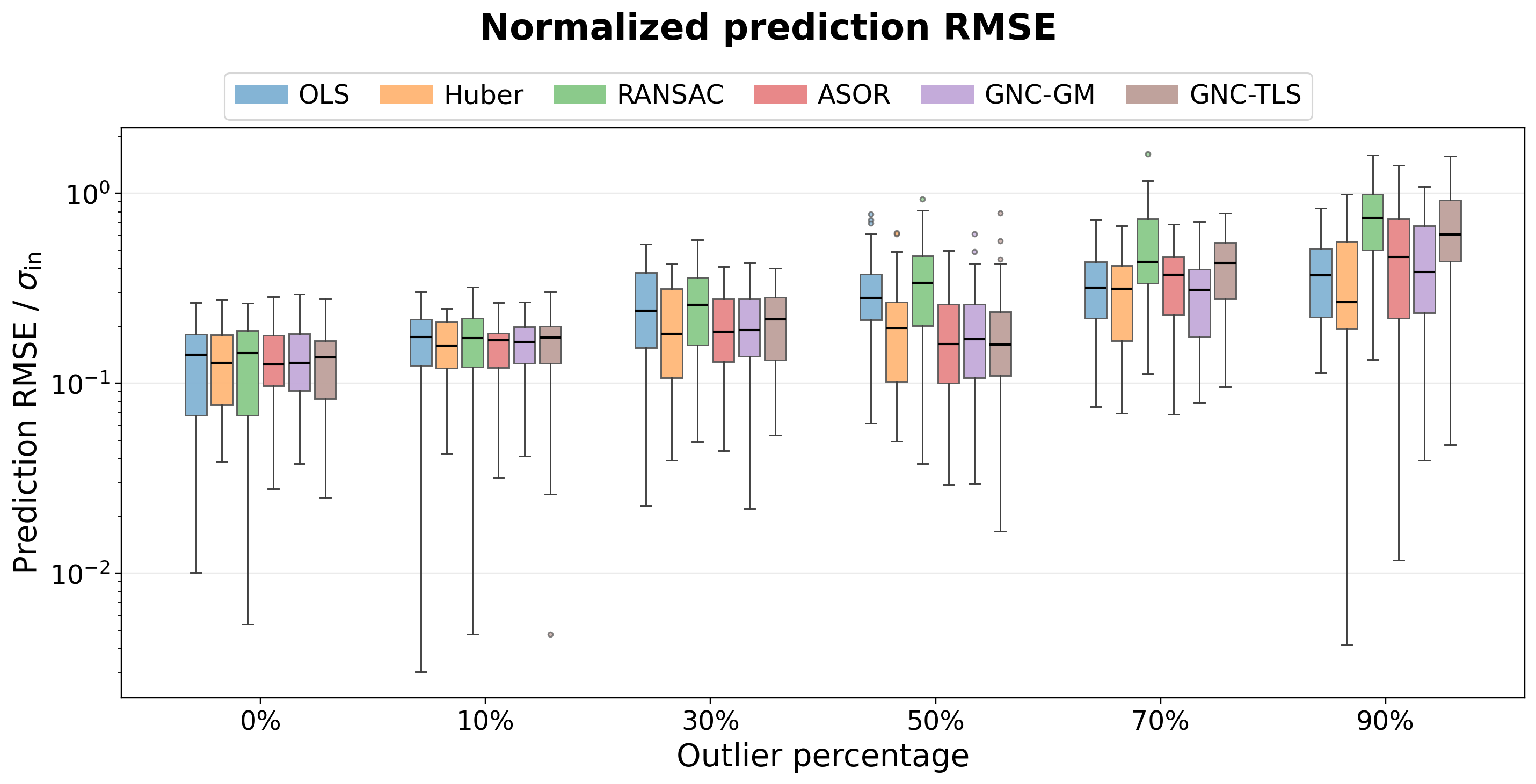
Figure 3 shows zero-mean Gaussian replacement outliers. Positive and negative errors partly cancel, so the estimated relationship is not consistently pushed in one direction. The robust estimators remain closely matched through moderate contamination, and OLS remains more accurate than it does under biased contamination.

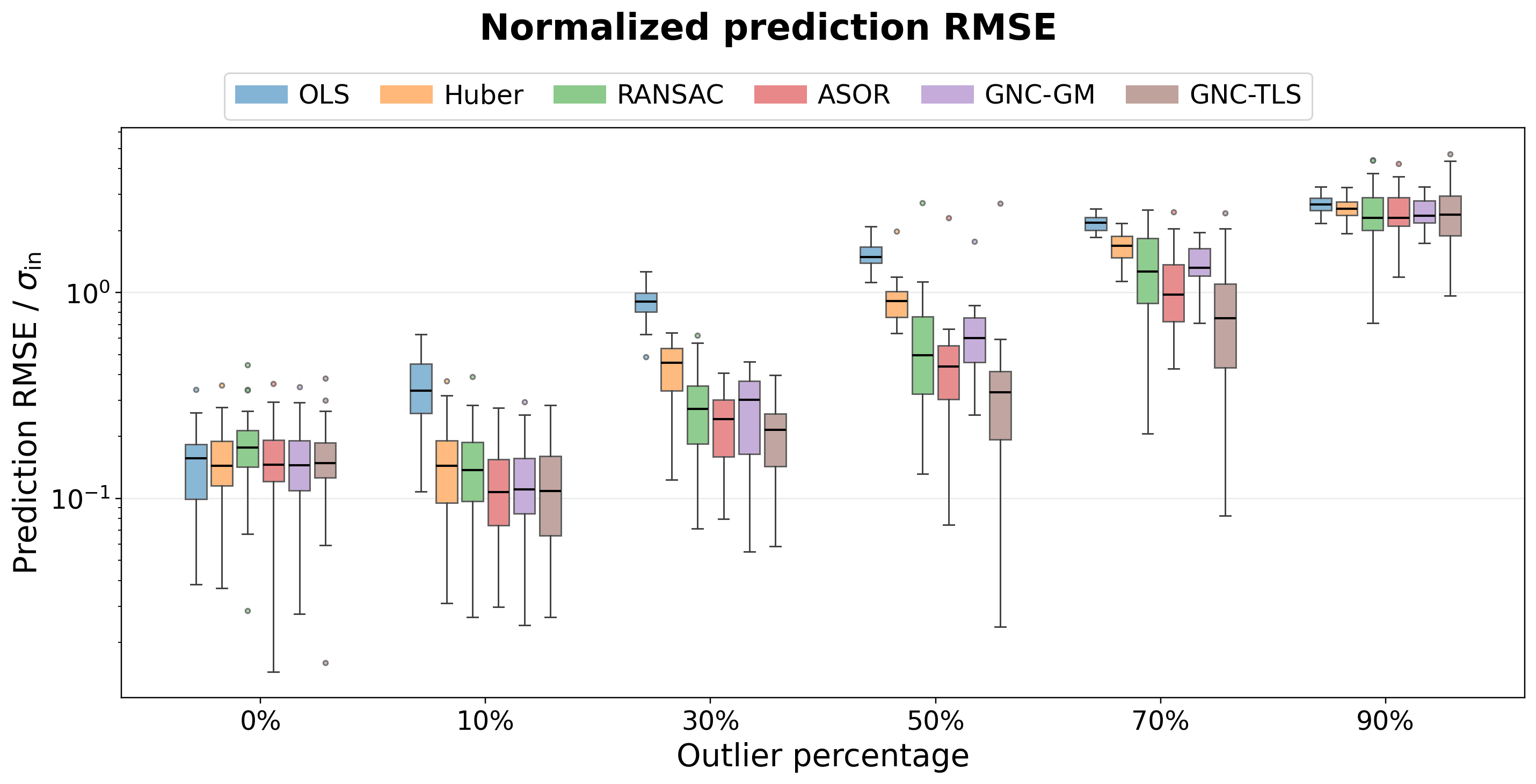
The pattern changes in Figure 4, where the outlier mean is shifted by $3sigma_{in}$

The important distinction is directional consistency. Zero-mean outliers inflate variability, but biased outliers repeatedly pull the fit in the same direction. OLS and Huber are affected most strongly; GNC-TLS and ASOR remain more accurate through moderate contamination. At 90%, the corrupted observations dominate, and the median errors of all six estimators become similar.

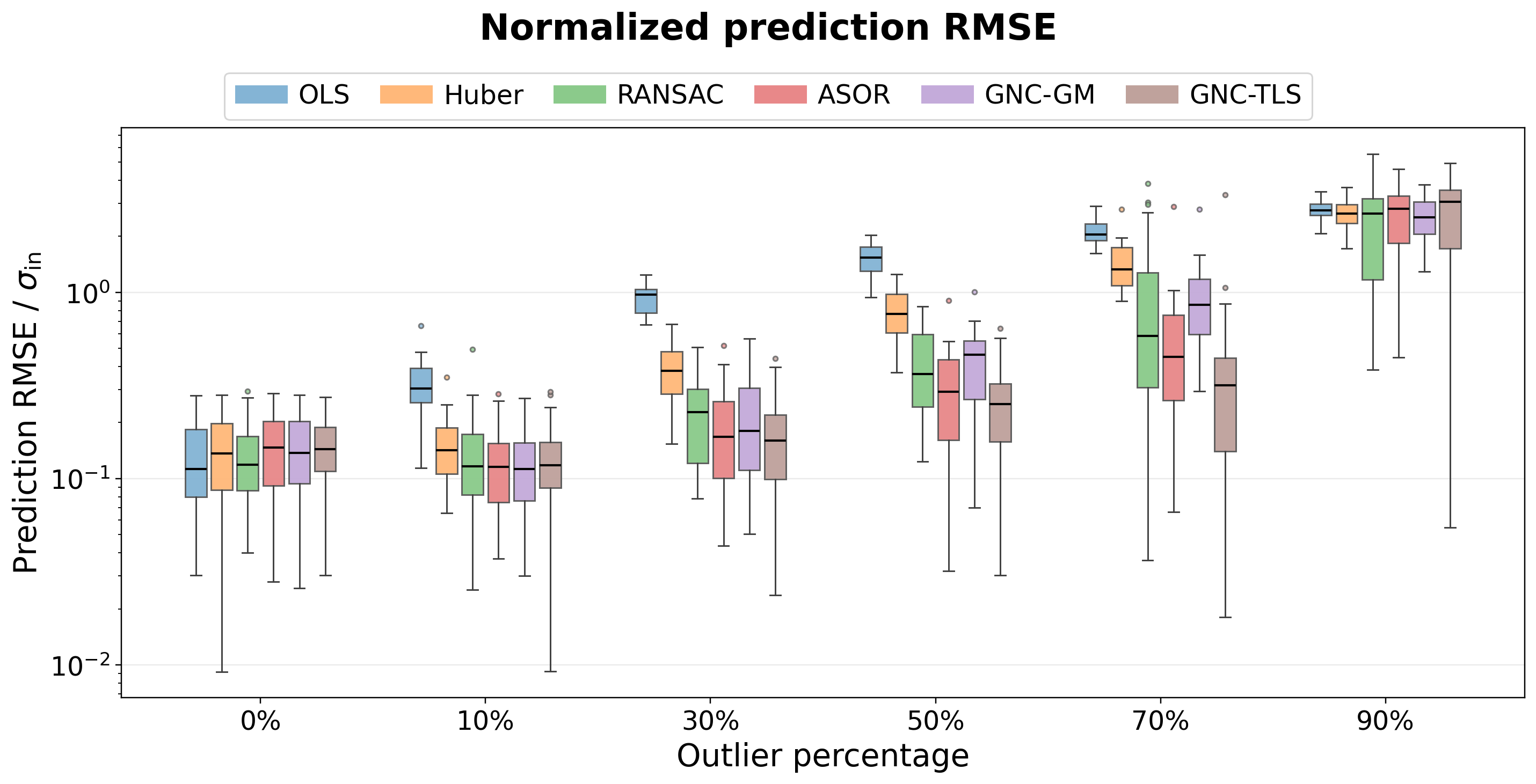
But is that pattern specific to Gaussian outliers? To check, Figure 5 repeats the experiment with a biased uniform distribution whose mean and variance are matched to the biased Gaussian case.

The broad ranking remains similar to the biased Gaussian case. At low outlier percentages, all robust estimators remain relatively accurate because the nominal observations still dominate the fit. As contamination increases, the differences become more pronounced: GNC-TLS and ASOR maintain the lowest prediction errors through moderate and high outlier levels, while OLS and Huber deteriorate more rapidly.

Finding 2: A coherent competing line is a model-identification problem

So far, the corrupted observations have been independent. The next experiment is harder: what happens when the outliers themselves form a coherent alternative model? Figure 6 evaluates outliers that follow a second line with five times the nominal slope.

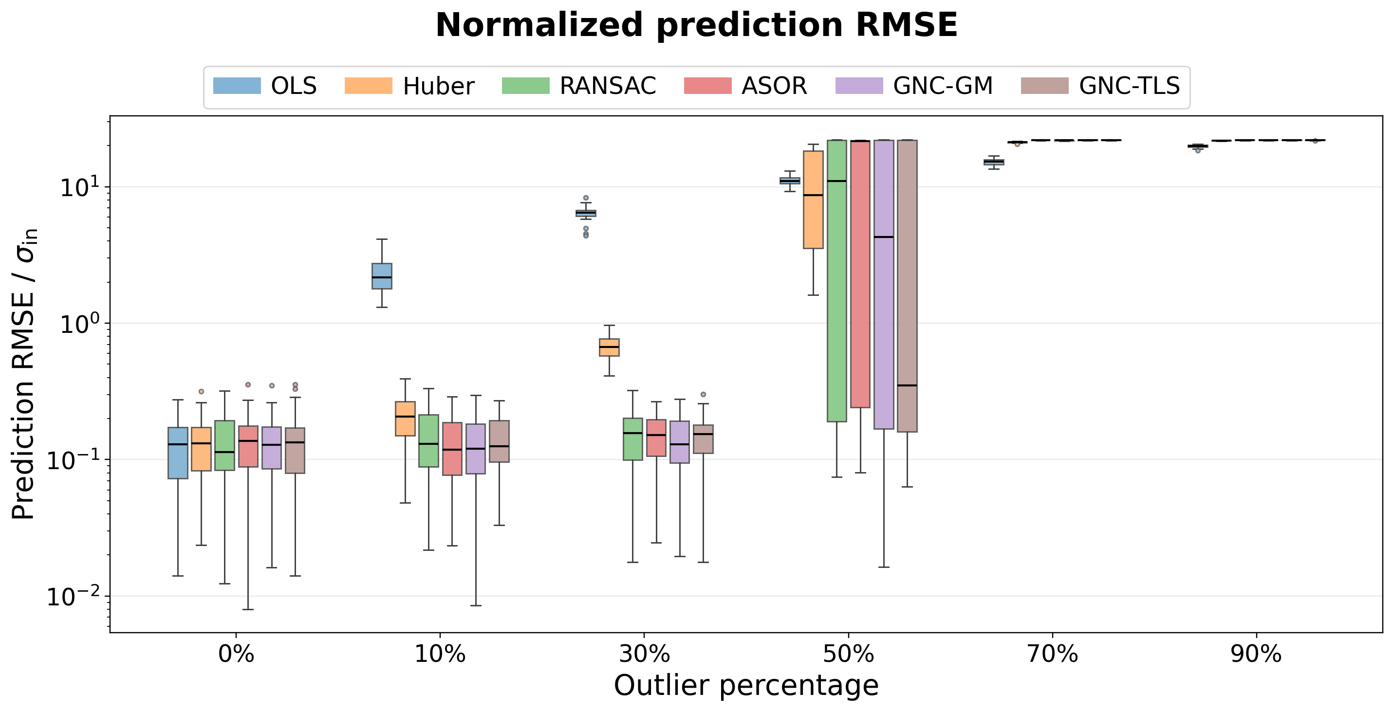
At 10% and 30%, the robust estimators recover the nominal relationship. At 30%, median normalized RMSE values are 0.157 for RANSAC, 0.152 for ASOR, 0.130 for GNC-GM, and 0.154 for GNC-TLS. Huber is less effective, while OLS is pulled strongly toward the competing line.

The problem becomes fundamentally ambiguous at 50% contamination, where the nominal and competing structures contain the same number of observations. The wide boxes indicate that different Monte Carlo realizations may lead robust estimators toward either of the two coherent relationships.

At 70% and 90%, the competing line is the dominant structure. The robust estimators generally select it, producing normalized RMSE values near 22 relative to the nominal model. This is an identifiability limitation, not merely a numerical failure. Without labels, physical constraints, temporal information, or a multi-model formulation, the data alone do not reveal which coherent relationship is the intended one.

Finding 3: Robustness requires additional computation

Accuracy is only one side of the story. Robustness requires additional computation, and the methods pay very different prices for it. Figure 7 shows runtime under biased Gaussian contamination.

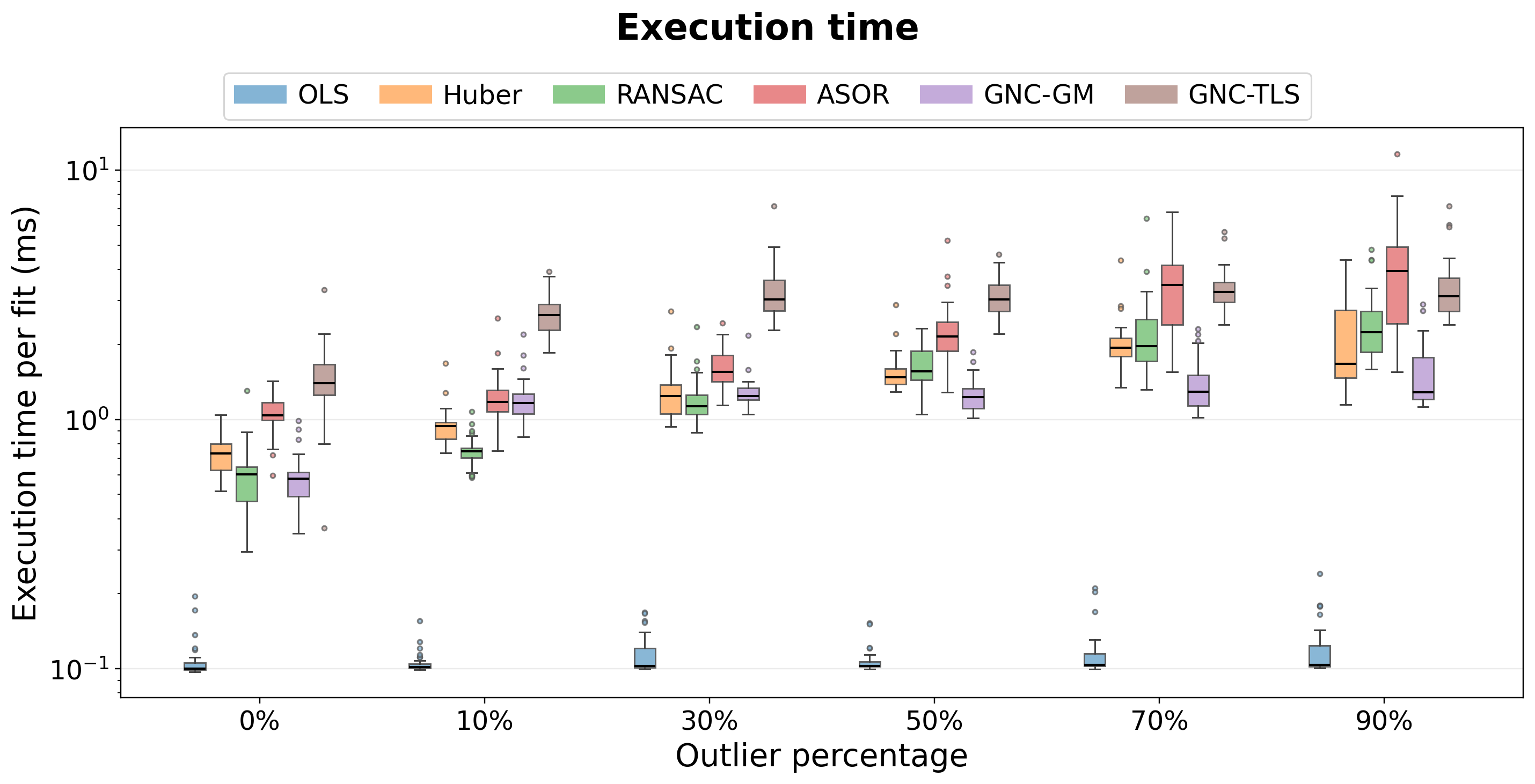
OLS remains fastest because it requires one least-squares solve. The robust estimators perform repeated weighted solves or evaluate multiple RANSAC hypotheses. GNC-GM generally provides the lowest and most stable iterative cost, while GNC-TLS is generally the most expensive because its continuation schedule requires more updates. ASOR occupies an intermediate accuracy–runtime region.

Absolute sub-millisecond timings depend on the processor, power mode, operating-system scheduling, Python version, and BLAS implementation. The relative ordering and scaling trends are more transferable than the exact millisecond values.

Table 3 provides a representative comparison across all four contamination models at 50% contamination.

Table 3. Median execution time in milliseconds at 50% contamination for N = 100 and 30 Monte Carlo realizations.

OLS remains substantially faster than the robust estimators. Among the iterative methods, GNC-GM generally has the lowest and most stable runtime. Huber, RANSAC, and ASOR have intermediate computational costs, whereas GNC-TLS is typically the most expensive because its continuation schedule requires multiple weighted least-squares solves.

The competing-line case produces an unusually large Huber runtime at 50% contamination, indicating slower convergence for this particular configuration. This isolated result should not be interpreted as a general runtime property of Huber regression.

Finding 4: More observations reduce variability, not systematic bias

A natural question is whether simply collecting more data makes the contamination problem disappear. Figures 8 and 9 fix biased Gaussian contamination at 50% and vary the sample size from 50 to 5000.

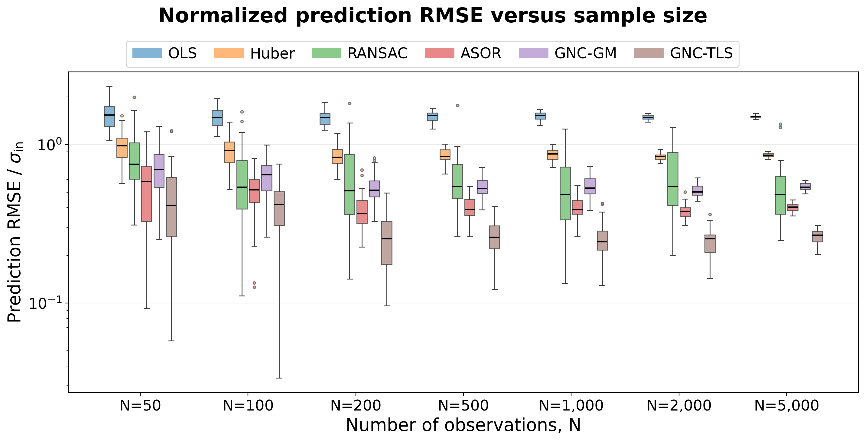
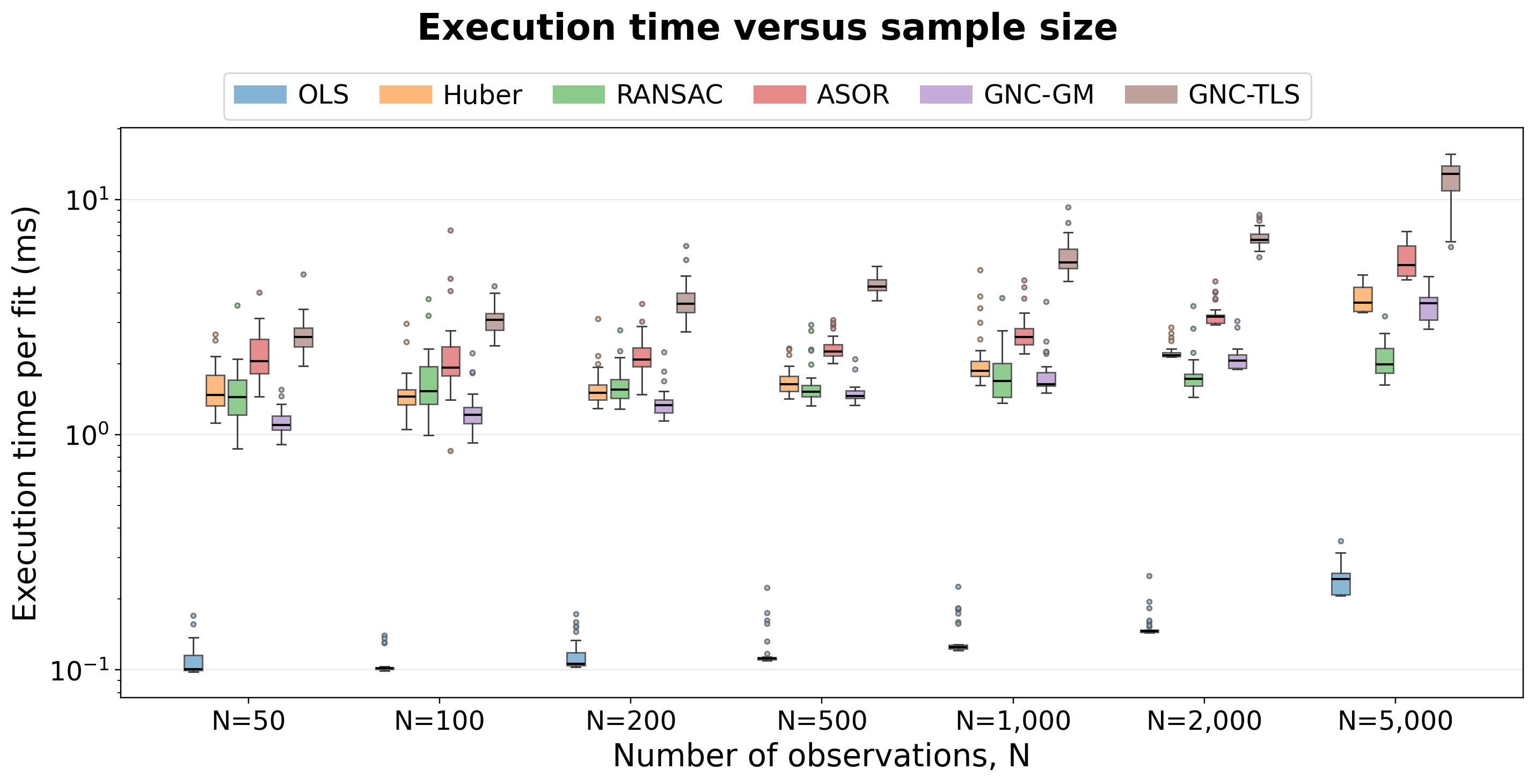
OLS remains biased as N increases: its median normalized RMSE is 1.533 at $N=50$

GNC-TLS has the lowest median error at every tested sample size. Its median decreases from 0.411 at $N=50$

Runtime increases with sample size. From $N=50$

RANSAC grows more slowly because its adaptive stopping rule evaluates a similar number of hypotheses across the tested sample sizes, although each hypothesis becomes more expensive as N increases.

Finding 5: Normalization preserves the ranking across noise scales

Finally, I change the absolute noise scale while preserving the relative contamination strength. This checks whether the observed ranking is tied to one particular measurement scale. The final experiment varies:$sigma_{mathrm{in}}^2 in {10, 100, 1000, 10000}$

Table 4. Median normalized prediction RMSE as the nominal-noise variance changes. Boldface marks the two lowest values in each column.

The normalized results remain broadly stable as$sigma_{mathrm{in}}^2$

The leading methods remain consistent across noise scales: GNC-TLS has the lowest median normalized error, followed by ASOR, whereas OLS has the largest error. The small variations between columns are consistent with finite Monte Carlo variation and show no systematic dependence on the absolute measurement scale.

Which estimator should you start with?

There is no universal winner. The right starting point depends on what you know about the data, how aggressively you are willing to reject observations, and how much computation you can afford. Domain knowledge, residual diagnostics, computational constraints, and sensitivity analysis should all inform the choice. Practical starting points are summarized in Table 5.

Table 5. Practical starting points for estimator selection.

The table is a starting point, not a decision rule. In practice, I would fit more than one robust estimator, compare the resulting coefficients and residual patterns, and test sensitivity to reasonable scale and threshold choices.

Agreement across methods increases confidence in the recovered relationship; strong disagreement is itself useful evidence that the data may contain multiple structures or that the assumed nominal-noise scale needs to be reconsidered.

What this benchmark does not establish

There are also clear limits to what these experiments tell us. This is a controlled scalar-regression benchmark, not a universal leaderboard for robust estimation. The benchmark studies a scalar linear model with one-dimensional residuals, known nominal noise, fixed algorithmic settings, and synthetic contamination.

Different conclusions may emerge for high-dimensional regression, leverage points in the predictor space, heteroscedastic noise, nonlinear models, correlated errors, or real datasets with unknown ground truth.

The runtime results are implementation- and machine-dependent. The experiments also do not solve model identification when multiple coherent structures are present. Robust residual weighting can suppress isolated corruption, but it cannot determine the intended model without additional information once an alternative structure dominates.

What should you take away from this?

The most useful lesson from these experiments is broader than the ranking of the six methods: the percentage of outliers alone does not determine how difficult a regression problem is. Zero-mean outliers can partly cancel, while biased observations repeatedly pull the estimate in the same direction. Even Gaussian and uniform outliers with matched first two moments can produce different errors. Distribution, bias, and structure all matter.

More data help with variability, but not necessarily with bias. When the same contamination mechanism persists, increasing the sample size does not make OLS converge back to the nominal relationship.

In these experiments, GNC-TLS achieved the strongest overall accuracy when aggressive rejection was beneficial, ASOR provided a favorable accuracy–runtime compromise, and GNC-GM offered relatively stable computational behavior. These rankings are useful, but they depend on the assumptions and contamination models used here; they should not be treated as a universal leaderboard.

The competing-line experiment gives the strongest warning. Once corrupted observations form a coherent alternative relationship, robust regression is no longer simply an outlier-rejection problem. It becomes a model-identification problem, and residual weighting alone cannot tell us which coherent structure is the one we intended to recover.

Since we rarely know exactly how outliers will appear in practice, robust estimators are best judged across several plausible contamination patterns, with both accuracy and computational cost in view.

Next in the series. The robust regression series continues with polynomial regression, extending the comparison to nonlinear relationships and higher model complexity.

References

1. Legendre, A. M. (1805). Nouvelles méthodes pour la détermination des orbites des comètes. F. Didot.

2. Huber, P. J. (1964). Robust Estimation of a Location Parameter. The Annals of Mathematical Statistics.

3. Fischler, M. A., and Bolles, R. C. (1981). Random Sample Consensus: A Paradigm for Model Fitting with Applications to Image Analysis and Automated Cartography. Communications of the ACM.

4. Yang, H., Antonante, P., Tzoumas, V., and Carlone, L. (2020). Graduated Non-Convexity for Robust Spatial Perception: From Non-Minimal Solvers to Global Outlier Rejection. IEEE Robotics and Automation Letters.

5. Chughtai, A. H., Tahir, M., and Uppal, M. (2024). Bayesian Heuristics for Robust Spatial Perception. IEEE Transactions on Instrumentation and Measurement.

Get in touch 👋

For more of my work, explore my GitHub, or connect with me on LinkedIn. I welcome questions, new ideas, and opportunities to collaborate in Data science, AI and Statistical Signal Processing. If you enjoy my articles, sharing them with others helps these conversations reach more people.