Guided Merge Sort : An Optimized Sorting that Picks the Best from Ordinary and Multi-Way Merge Sort Algorithms

Introduction

In this article, I am going to present a novel approach for merging several sorted sequences into one called guided K-merge and, based on that, a general-purpose sorting algorithm called guided K-merge sort.

The current approaches to efficient merging of several sorted sequences require some helper data structures, such as a sorted array or a priority queue. In contrast, guided K-merge keeps the required information with the help of multiple isomorphic code fragments, and uses the goto operator to jump between them.

Theoretical evaluation shows that guided K-merge reduces the time for such a multi-way merge, compared to the current implementation that uses a sorted array. At the same time, guided K-merge doesn’t introduce any overhead, in contrast to the current implementation that uses a priority queue.

Based on all that, the practical evaluation shows that depending on the type of data being sorted, guided K-merge sort can perform up to 15% faster, compared to the widely used merge sort algorithm.

This article is organized as follows:

···

1. Recalling merge, merge sort, and K-merge sort algorithms

Sorting a sequence of values is an essential procedure in Computer science. Given an arbitrary sequence, after running any sorting algorithm on it, we expect all its values to be rearranged – most of the time in increasing order:

The necessity to sort arises, for example, when we need to:

• efficiently navigate over large volumes of data, and find necessary items there;

• present existing data to the end-users in a clearer way;

• identify certain patterns in large volumes of data;

• … and in many other cases arising in different fields.

There are different sorting algorithms, most famous of which are probably bubble sort, quick sort, and merge sort, each having its relatively strong and weak sides.

Merge sort (or some variation of it) is often the default sorting algorithm in standard libraries of various programming languages. For example:

• Java uses merge sort when sorting an array of non-primitive data types,

• Python uses Timsort, which is a combination of merge sort and insertion sort algorithms,

• C++ uses merge sort (or some variation of it) when the sorting must be stable.

Recalling the merge sort algorithm

Understanding the merge procedure and merge sort algorithm is important for proceeding with this article. There are many good tutorials and videos on the Web, such as [1], [2] and [3]. This sub-section will also help recall them.

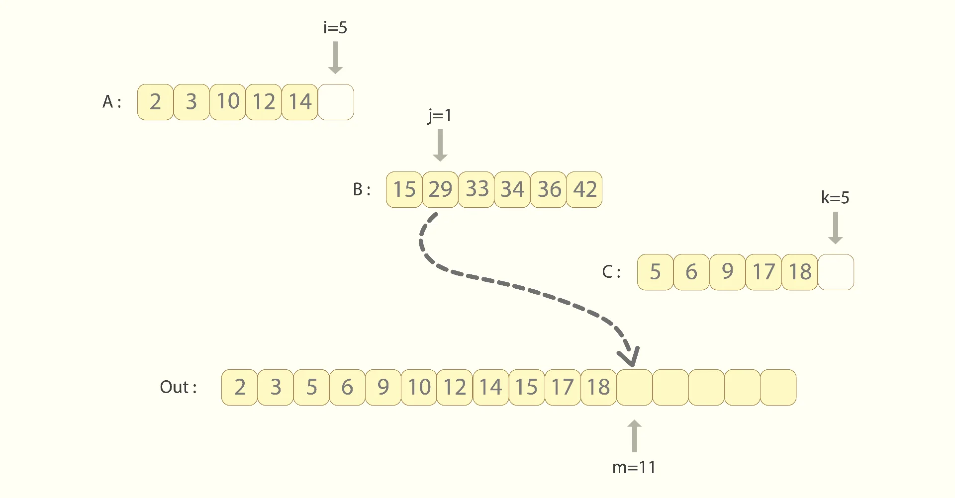
Merge sort is a recursive algorithm, the building block of which is the merge procedure. Given two already sorted sequences, the purpose of merge is to combine them into one, preserving the sorted state in the result:

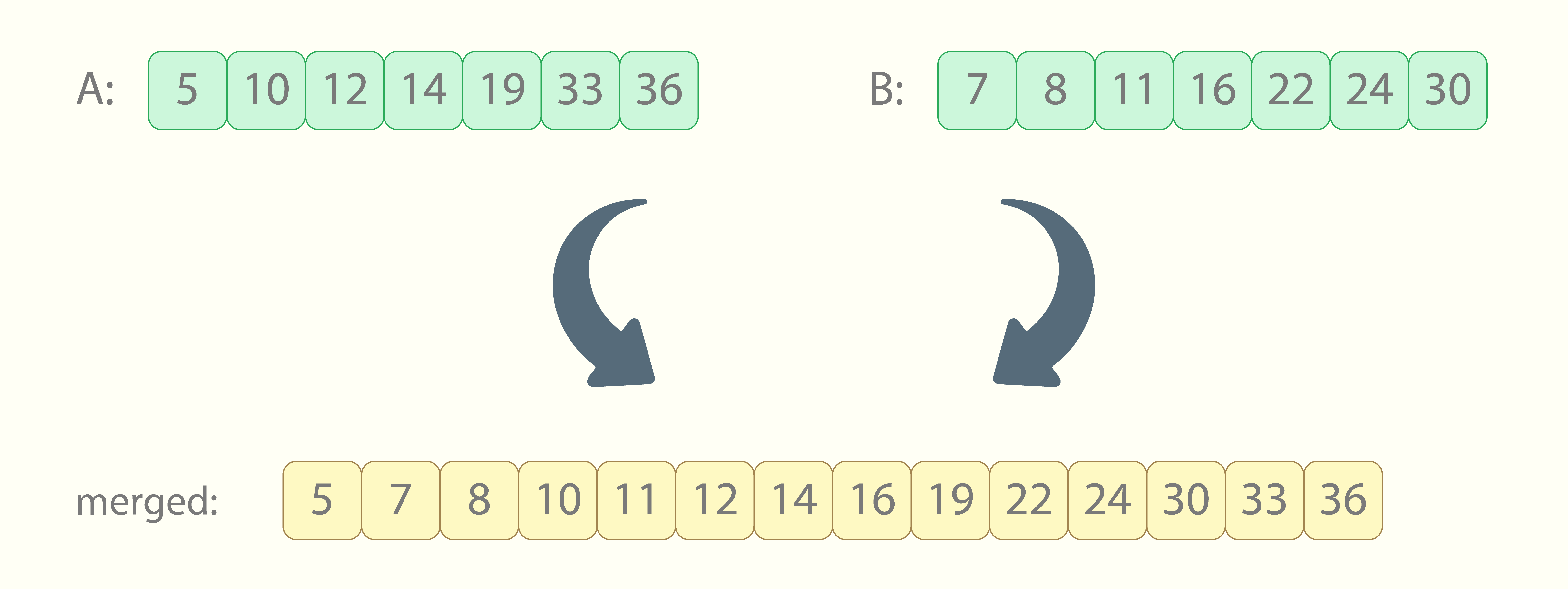
Within the merge procedure, both input sequences ‘A’ and ‘B’ arrive in sorted order. This means that after the merge, values of ‘A’ will preserve their relative order in the output sequence, as well as values of ‘B’ will:

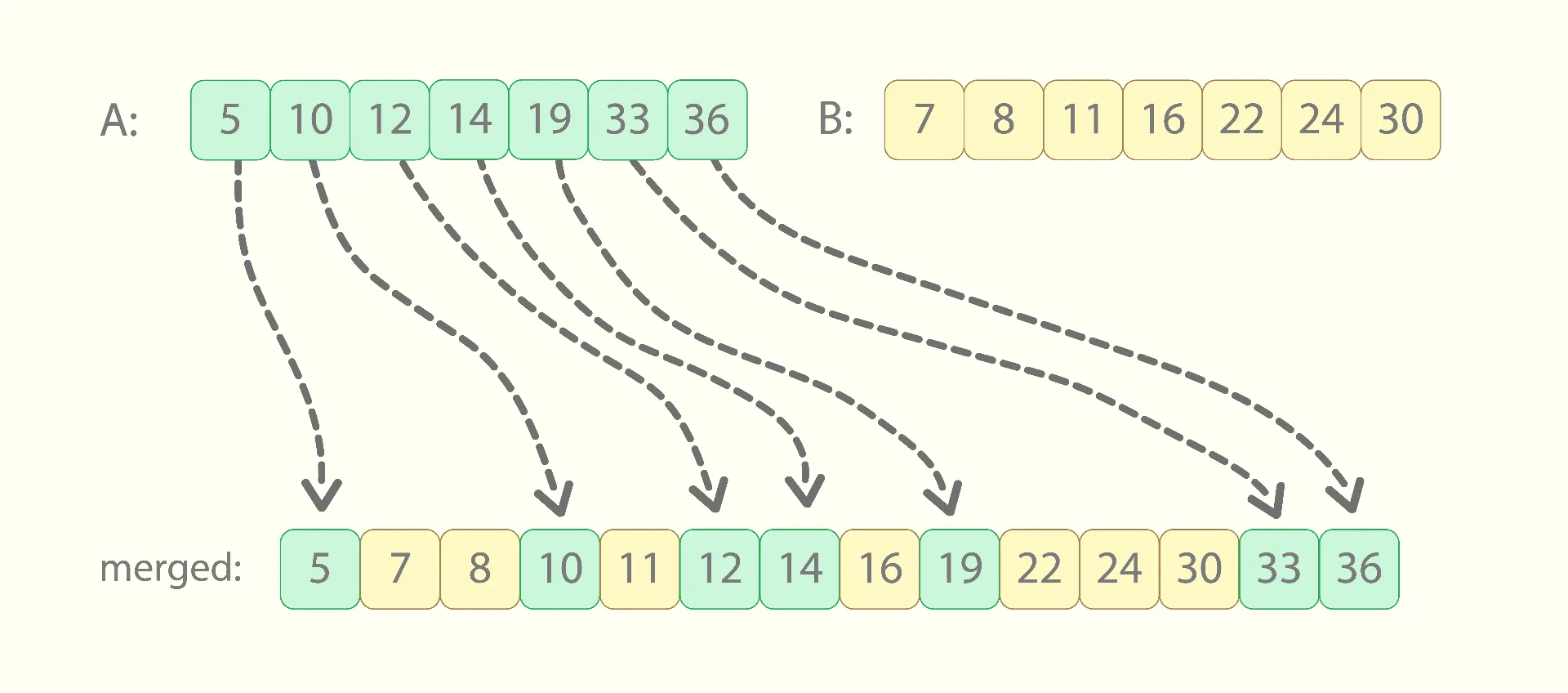
This fact allows us to produce the output sequence from left to right, while scanning both input sequences in parallel, also from left to right.

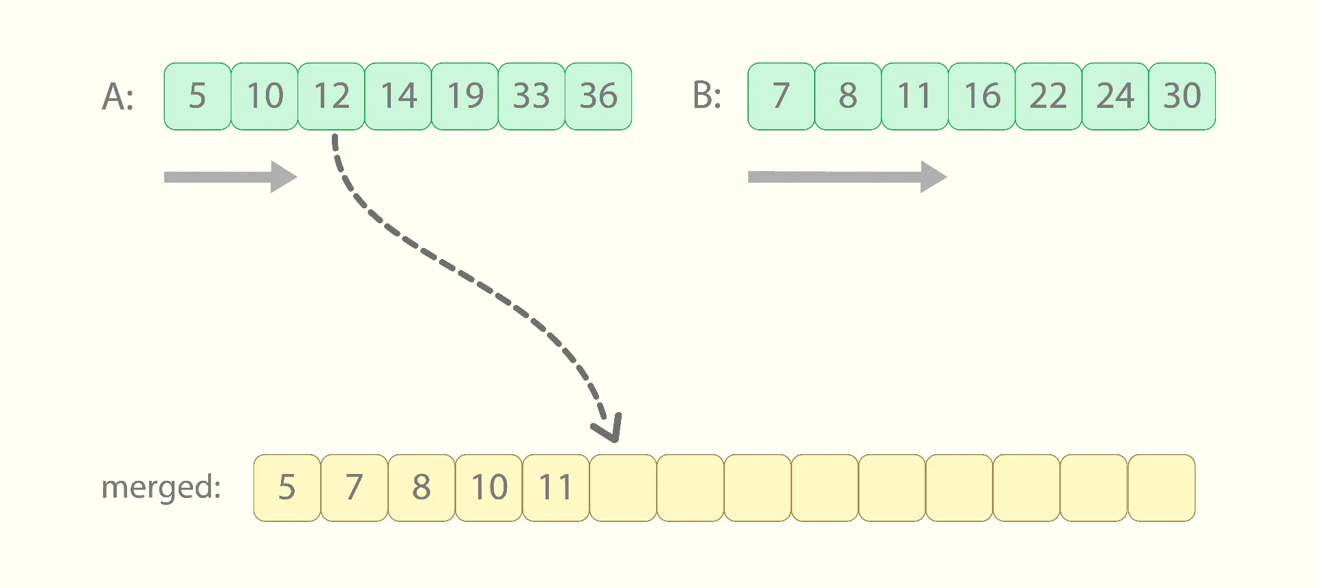
At every step, we will just compare the next value of ‘A’ with the next value of ‘B’, and take the smaller one into ‘Out’.

Close to the finish, one of the sequences will be completely moved to the output, while some short fragment will remain in the other one. It means the values of the remaining fragment are greater than all the values already considered, so we can just copy it to the output.

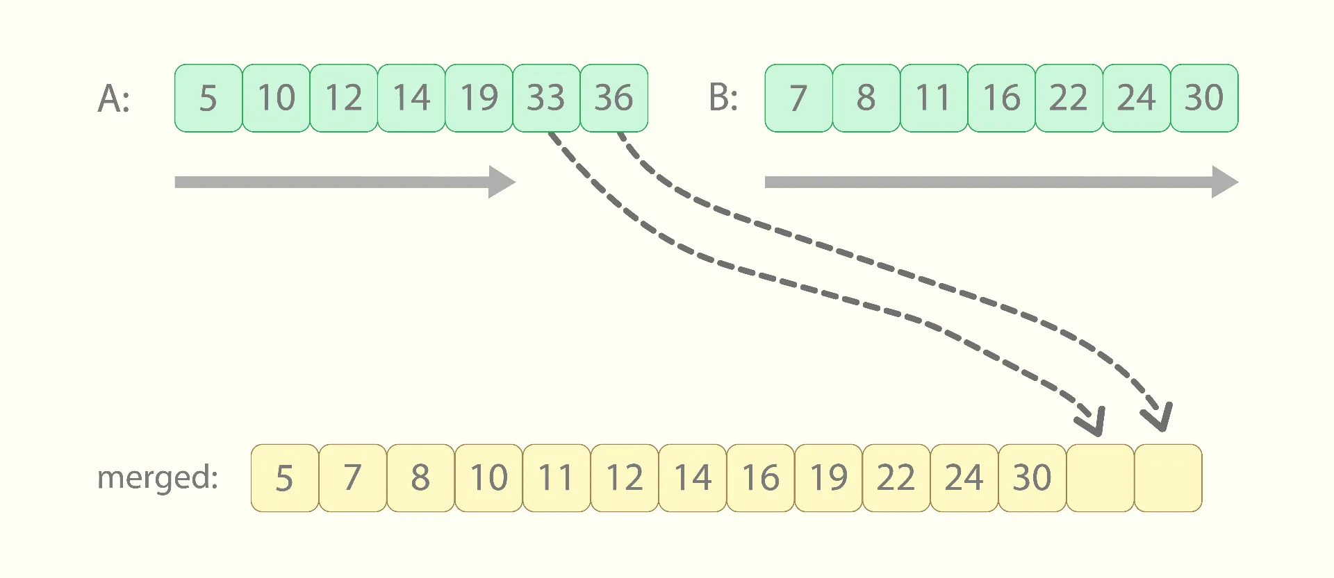
The code for the merge procedure in C++ becomes:

/// Merges two sorted arrays ‘A’ and ‘B’ into result array ‘Out’./// ‘n1’ and ‘n2’ are the lengths of arrays ‘A’ and ‘B’, respectively.void merge( const int A[], int n1, const int B[], int n2, int Out[] ) {	int i=0, j=0, m=0;  // Indexes over arrays ‘A’, ‘B’ and ‘Out’.	while ( i < n1 && j < n2 ) {  // We still have two arrays (tails) to merge		if ( A[i] < B[j] )			Out[m++] = A[i++];  // Next value of ‘A’ is appended to ‘Out’		else			Out[m++] = B[j++];  // Next value of ‘B’ is appended to ‘Out’	}	// One array is exhausted, so it remains     // to copy the tail of the other array to ‘Out’	if ( i == n1 )		std::copy( B+j, B+n2, Out+m );  // Append the tail “B[j..n2)” to ‘Out’	else		std::copy( A+i, A+n1, Out+m );  // Append the tail “A[i..n1)” to ‘Out’}

The time complexity of merge is always O(n₁+n₂), where ‘n₁’ and ‘n₂’ are the lengths of the input sequences. That’s because all the “n₁+n₂” values need to be copied (or moved) to the output, and every copy is performed in a constant amount of time.

Now, the merge procedure outputs a sorted sequence, but it requires the input sequences to be sorted too. How can we use merge then to sort an arbitrary input array? The answer is: using recursion, and that is how the merge sort algorithm operates. What it does to sort an n-long input sequence is:

• divides it into 2 equal parts (halves),

• recursively sorts each half, in an independent manner,

• merges the sorted halves into the result array.

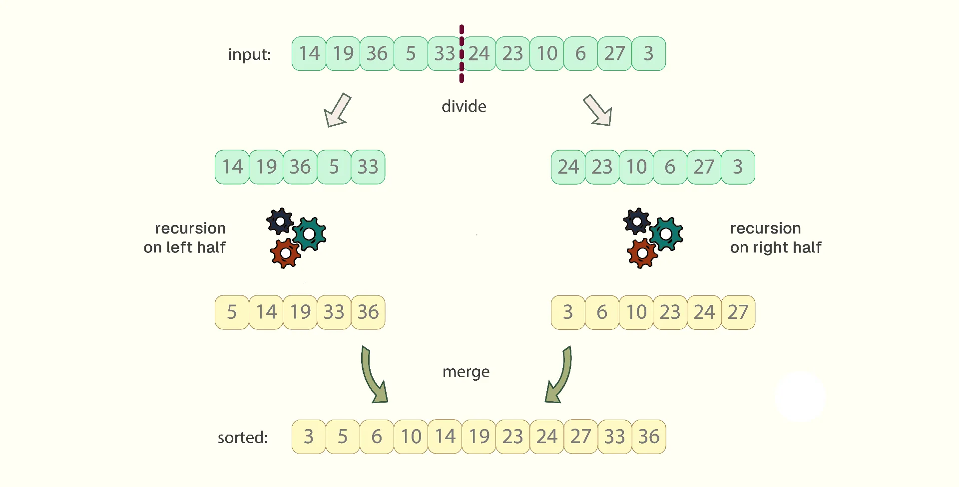
This means that, when recursively sorting the left half, it will also be divided into 2 equal parts (each being a quarter now), each of which will be sorted recursively, before being merged into the sorted left half. The same also refers to the right half of the sequence.

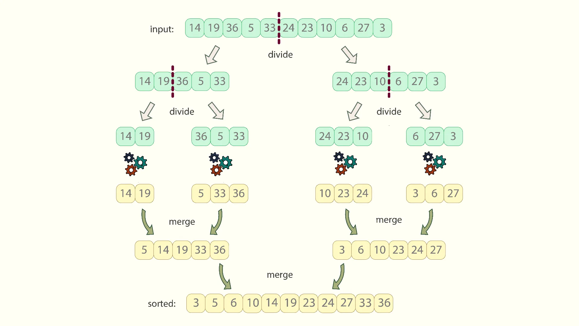
This way, while recursion deepens, the current sub-array that should be sorted is shortened twice. The recursion stops when the algorithm reaches a 1-element sub-array, which, obviously, does not require any sorting. Some optimizations stop recursion sooner, once the current sub-array becomes shorter than a predefined threshold, after which they switch to a simpler sorting algorithm, often to insertion sort.

The code of the merge sort algorithm in C++ becomes:

/// Sorts the n-long array ‘X’, in an increasing order.void merge_sort( int X[], int n ) {	// Check exit branch first	if ( n < 16 ) {		// According to a common practice of various sorting 		// algorithms, here also we switch to Insertion sort once 		// the length of sub-array becomes small enough.		insertion_sort( X, n );		return;	}	// Otherwise, divide the n-long range into 2 equal parts	const int half = n / 2;	// Recursively sort each part	//    Note, because of the rounding in division by 2, the second 	//    part might result in a shorter length.	merge_sort( X, half );	merge_sort( X+half, n-half );	// Temporarily allocate a buffer for storing the result of the merge.	//    Note, in an optimal implementation it makes sense to allocate 	//    buffer only once, and use it in every recursive call. We just 	//    don’t do that here for simplicity.	int* buffer = new int[ n ];	// Merge the 2 sorted arrays into one	merge( X, half, 			X+half, n-half, 			buffer );	// Copy back the merged sequence from buffer to original array	//   Note, in an optimal implementation we should use ping-pong 	//   merge sort, thus merging the data to buffer on even levels 	//   of recursion, and merging it back from buffer to ‘X’ on 	//   the odd levels of recursion. That significantly reduces the 	//   time spent on copying-back from buffer. We just don’t do it 	//   either, again for simplicity.	std::copy_n( buffer, n, X );	delete [] buffer;}

As we see, merge sort uses a temporary buffer to store the output of the merge procedure. This is required, as we can’t write the merged sequence into the same memory location from which we read either of its input sequences ‘A’ or ‘B’. That’s why, on every invocation of “merge_sort”, first we write the merged sequence into the temporary buffer, and then copy it back to the original array ‘X’.

There is an optimization called ping-pong merge sort, which, when applied, eliminates such copying back almost entirely. It does that by repeatedly swapping the roles of ‘X’ and ‘buffer’. Briefly speaking, on the even levels of recursion it merges intermediate results from ‘X’ to ‘buffer’, while on the odd levels of recursion it merges them from ‘buffer’ back to ‘X’. However, for simplicity, we don’t implement the ping-pong optimization in this paper.

Recalling the K-merge sort algorithm

The algorithm that I am going to describe is in fact an optimization of one variation of merge sort, which is called K-merge sort. The difference between merge sort and K-merge sort is in how many equal parts the sequence is divided into. If merge sort always divides it into 2 parts, then what K-merge sort does is:

• divide the input sequence into K equal parts,

• recursively sort them in an independent way (applying K-merge sort to each of those parts),

• combine the K sorted sequences into one, using the K-merge procedure.

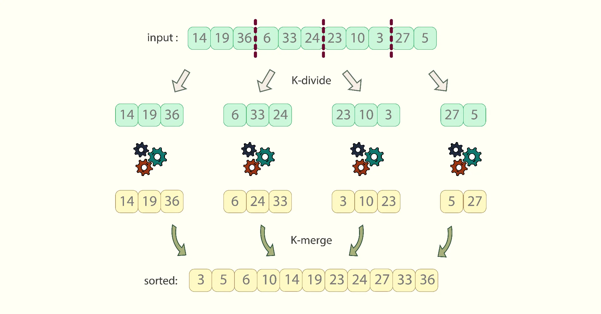
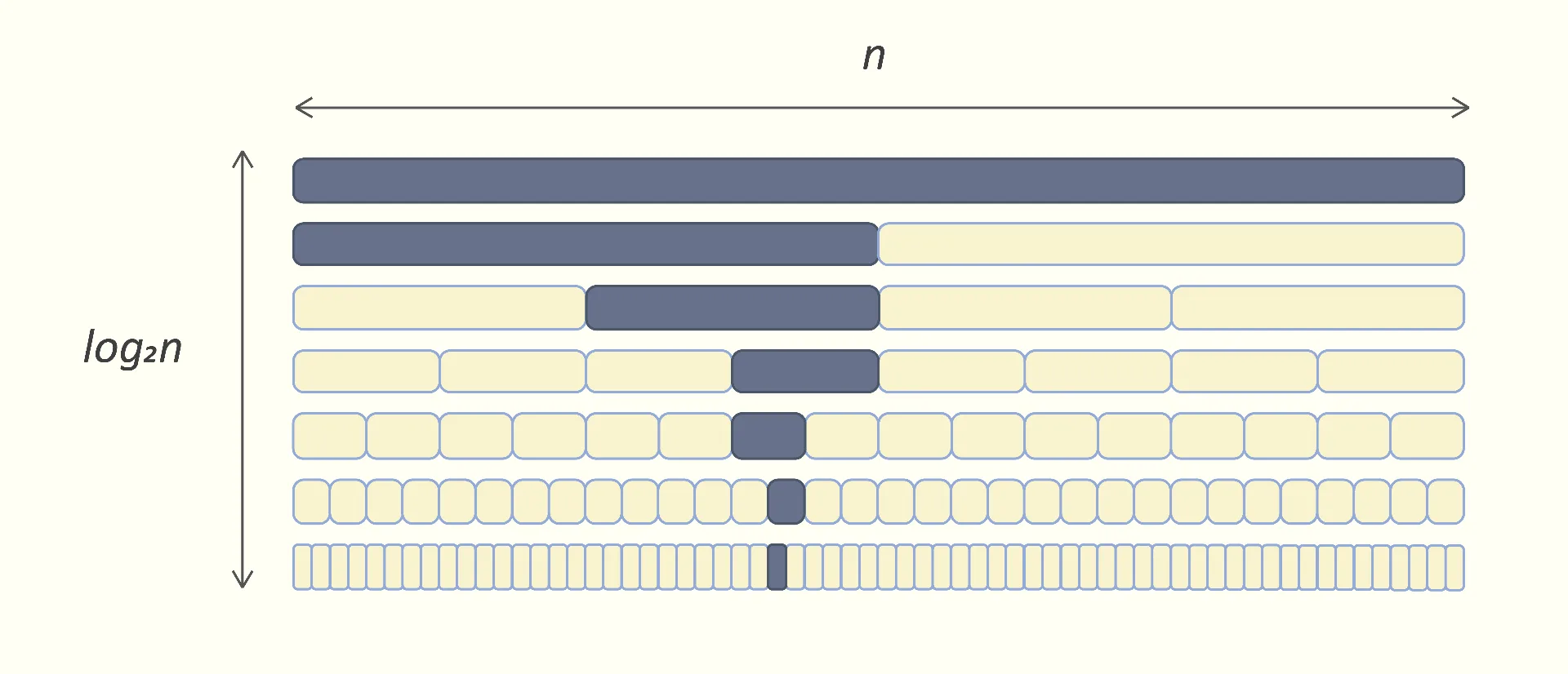
The advantage of K-merge sort over ordinary merge sort is the decrease in recursion depth. On every level, merge sort splits the current range into halves, which, for an n-long input sequence, requires “log₂n” levels to reach the 1-long sub-range, thus, to reach the exit branch of recursion:

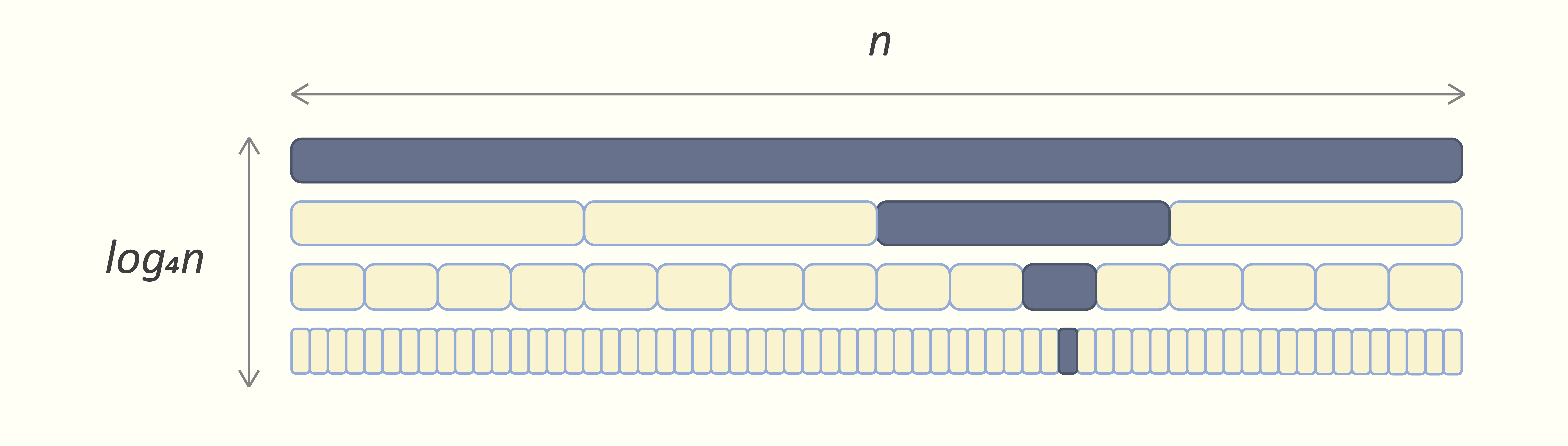
While K-merge sort always cuts the current range into K equal parts, it will require only “log_Kn” levels to bring the initial n-long input sequence to 1-long ranges:

Within K-merge sort, as the depth of recursion decreases, so does the overall number of value assignments. We can observe this with the help of the following diagrams: for ordinary merge sort, its complete workflow can be depicted like this:

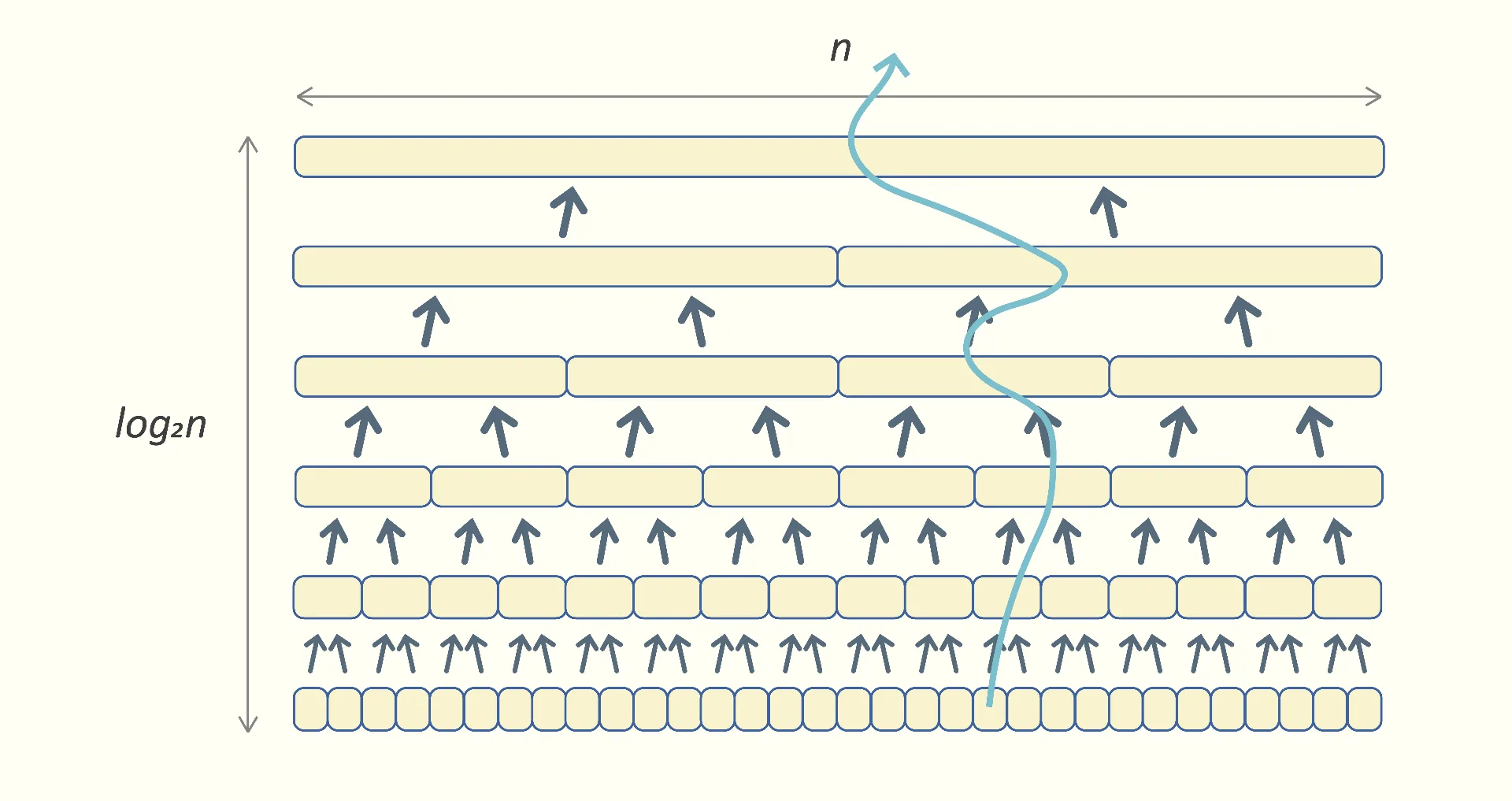
According to the figurative arrows, the number of times every value is assigned is proportional to “log₂n”. Thus, the number of assignments during the entire algorithm becomes proportional to “n*log₂n”, which makes the time complexity of merge sort O(n*log n).

For the K-merge sort algorithm, the complete workspace becomes shorter:

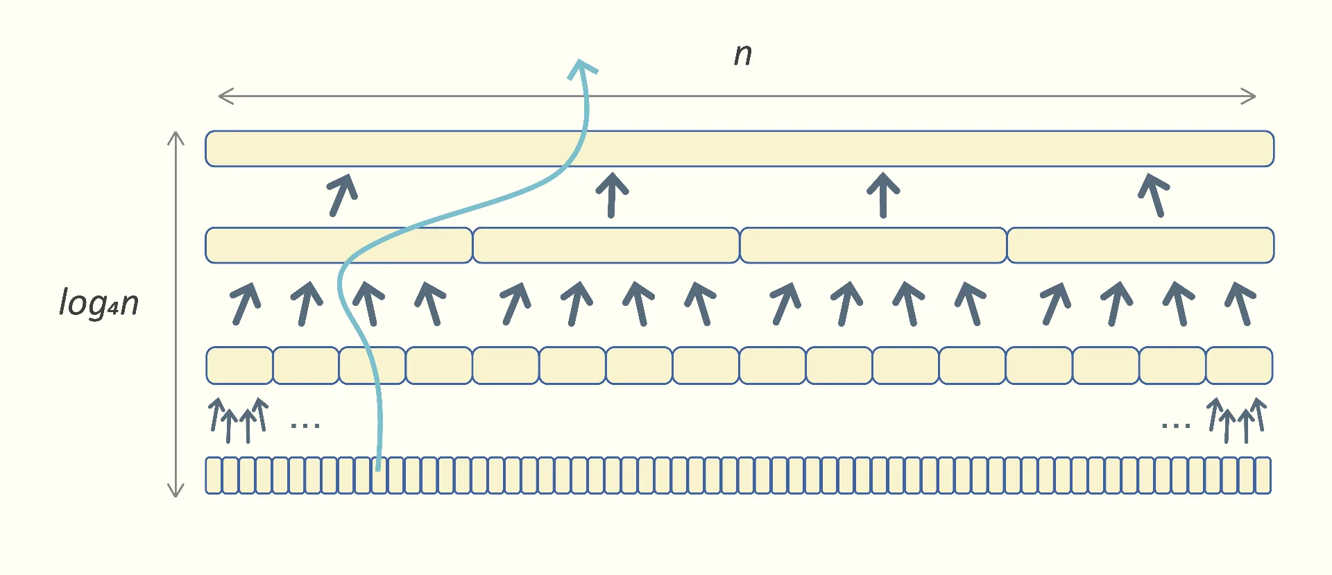
The number of times every value is being assigned now is proportional to “log_Kn”. Thus, the number of assignments during the entire K-merge sort becomes proportional to “n*log_Kn”.

We might wonder why K-merge sort is not the default sorting algorithm and is not widely preferred over merge sort.

The answer is that K-merge sort has also one drawback: merging ‘K’ sorted arrays requires more computation. When merging 2 arrays ‘A’ and ‘B’, at every step it is enough to compare the next value of ‘A’ with the next value of ‘B’, and copy the smaller one into the result. That’s why the code of the merge routine observed earlier was that short.

While when it comes to K-merge, in order to understand which value should go next to the result array ‘Out’, we should do more comparisons. Let’s assume “K=4”, so we are doing “4-merge”. To pick the smallest value from the next 4 input ones – “A[i]”, “B[j]”, “C[k]”, and “D[l]”, we should perform 3 comparisons now (please don’t confuse the lowercase ‘k’, which is the index over array ‘C’, with the uppercase ‘K’, which is the number of parts the sequence is being split into):

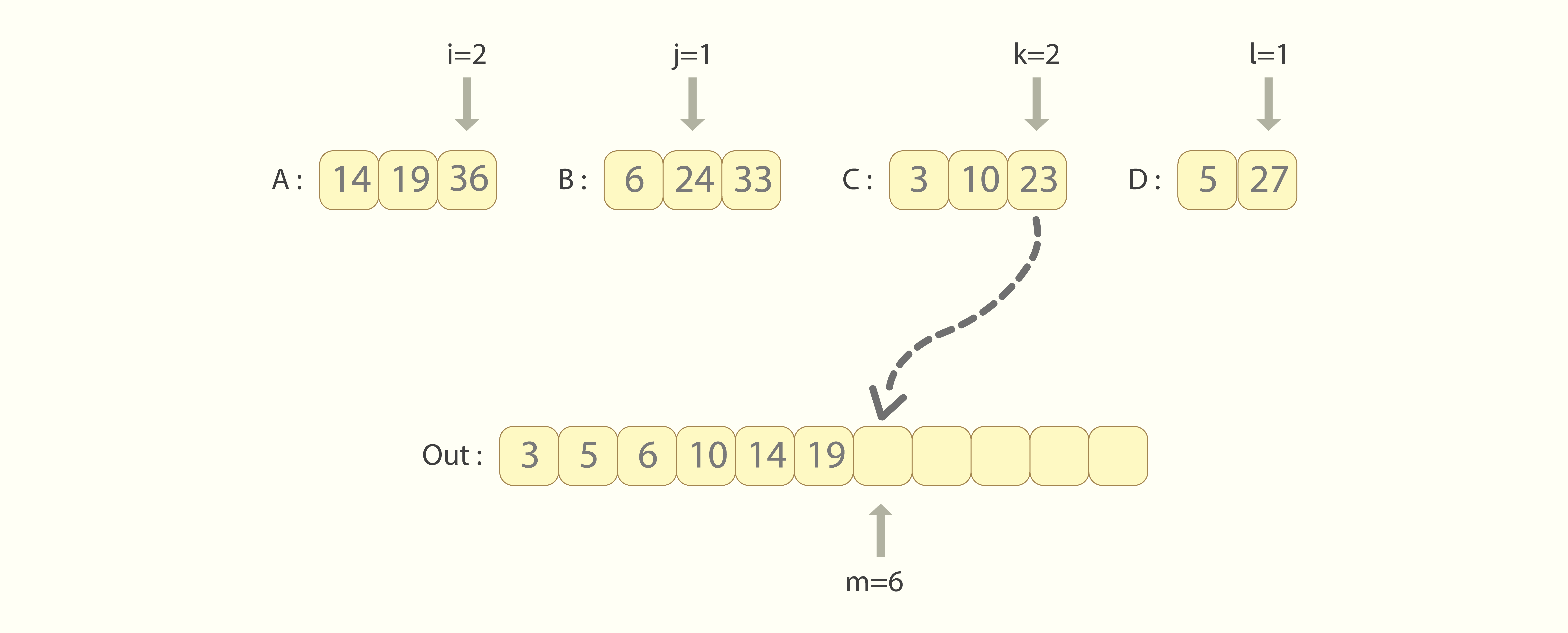
The code of the 4-merge procedure turns out significantly longer:

/// Merges four sorted arrays ‘A’, ‘B’, ‘C’ and ‘D’ into result array ‘Out’./// ‘n1’, ‘n2’, ‘n3’ and ‘n4’ are the lengths of the input arrays.void _4_merge( const int A[], int n1, const int B[], int n2, 		const int C[], int n3, const int D[], int n4, 		int Out[] ) {	int i=0, j=0, k=0, l=0, m=0;  // Indexes over arrays ‘A’, ‘B’, ‘C’, ‘D’                                   // and ‘Out’.	while ( i < n1 && j < n2 && k		// We still have four arrays (tails) to merge		if ( A[i] < B[j] ) {			// B[j] is certainly not the smallest			if ( A[i] < C[k] ) {  // C[k] is also not the smallest				// Remains to compare ‘A[i]’ and ‘D[l]’				if ( A[i] < D[l] )					Out[m++] = A[i++];				else					Out[m++] = D[l++];			}			else {  // A[i] is also not the smallest				// Remains to compare ‘C[k]’ and ‘D[l]’				if ( C[k] < D[l] )					Out[m++] = C[k++];				else					Out[m++] = D[l++];			}		}		else {			// A[i] is certainly not the smallest			if ( B[j] < C[k] ) {  // C[k] is also not the smallest				// Remains to compare ‘B[j]’ and ‘D[l]’				if ( B[j] < D[l] )					Out[m++] = B[j++];				else					Out[m++] = D[l++];			}			else {  // B[j] is also not the smallest				// Remains to compare ‘C[k]’ and ‘D[l]’				if ( C[k] < D[l] )					Out[m++] = C[k++];				else					Out[m++] = D[l++];			}		}	}	// One array is exhausted, so it remains to merge tails of the 3 others	if ( i == n1 )  // Array ‘A’ is exhausted		_3_merge( B+j, n2-j, C+k, n3-k, D+l, n4-l, Out+m );	else if ( j == n2 )  // Array ‘B’ is exhausted		_3_merge( A+i, n1-i, C+k, n3-k, D+l, n4-l, Out+m );	else if ( k == n3 )  // Array ‘C’ is exhausted		_3_merge( A+i, n1-i, B+j, n2-j, D+l, n4-l, Out+m );	else  // ‘D’ is exhausted		_3_merge( A+i, n1-i, B+j, n2-j, C+k, n3-k, Out+m );}

We see that along with the nested conditions, always 3 comparisons are required to figure out the smallest head value between ‘A[i]’, ‘B[j]’, ‘C[k]’ and ‘D[l]’. Generalizing, at every step the K-merge sort performs “K-1” comparisons to find the smallest one from the ‘K’ current head values.

The cost of doing more comparisons compensates the advantage of making fewer assignments. That is the reason the simpler merge sort is preferred over K-merge sort in practice. However, K-merge sort might be preferred in other circumstances, for example in external sorting (sorting outside of the RAM), where the cost of comparing 2 entries is much less than the cost of copying (or moving) them.

Actually, there is one more approach too for merging ‘K’ sorted arrays. There, all the current head values are stored in a specialized data structure, like a priority queue, which enables fast retrieval of the smallest head value in O(1) time, and its substitution with the next value in O(log K) time. A detailed description of this approach can be found at [4]. However, using such sophisticated structures always introduces significant overhead. For example, if the priority queue is implemented as a binary heap, the overhead will come from:

• making swaps during sift–up and sift–down operations,

• checking not to go beyond the physical range of the tree, and finally,

• allocating necessary space in dynamic memory.

That is the reason why a priority queue is generally not used for merging only a few (“K=3” or “K=4”) sorted sequences, as the mentioned overhead will certainly exceed possible gain in performance. Using a priority queue is justified when merging at least dozens of sorted sequences.

···

2. The guided merge procedure

In this article, I will describe the guided merge sort algorithm, which is based on the guided merge procedure. This is similar to how ordinary merge sort is based on the merge procedure. So we will discuss guided merge first.

In fact, both guided merge and guided merge sort concepts belong to the approach where we divide the current range into ‘K’ equal parts, not 2. So, to be more precise, they should be called guided K-merge and guided K-merge sort respectively. However, sometimes I prefer to omit the prefix “K” to make the naming more compact and easily pronounceable.

In this chapter we will observe the case when “K=4”, so we will be merging 4 sorted input sequences – “A”, “B”, “C” and “D”. As we already recalled, to do that K-merge algorithm repeatedly looks for the next smallest value between all the current heads (performing 3 comparisons per step), and appends it to the result sequence.

What if we act differently? What if instead of looking for the next smallest value from scratch, we always keep in memory how the K current head values are ordered in relation to each other? In our example, at the very first step, those 4 head values are “A[0]”, “B[0]”, “C[0]”, and “D[0]”, and their relative ordering is:

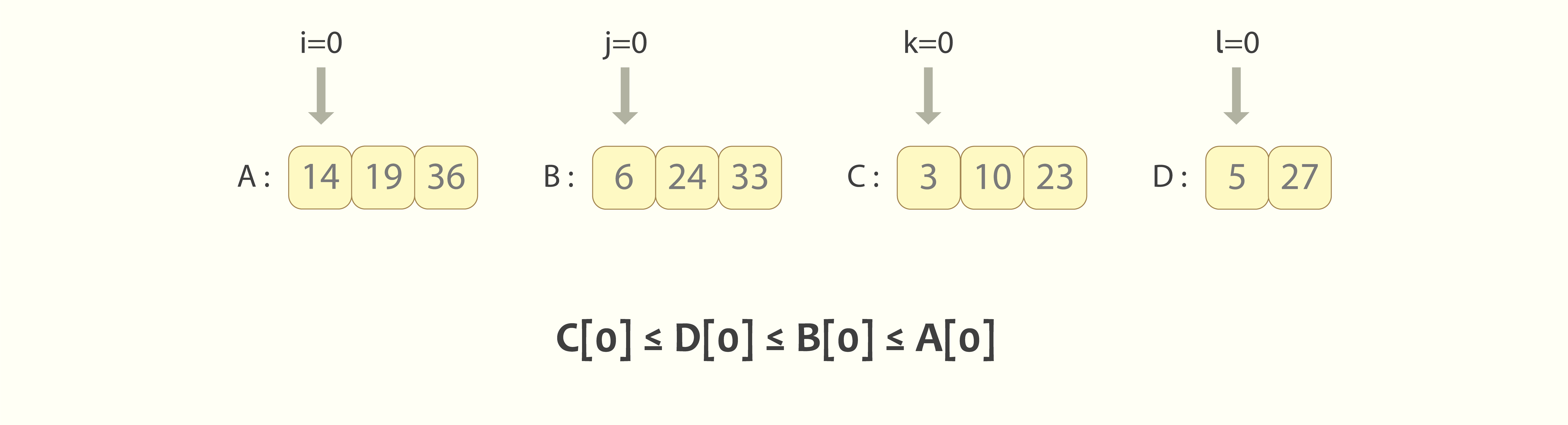
Having this, it is straightforward that the initial smallest value is the leftmost one among them – “C[0]”, and it should be taken to the result sequence first. However, once “C[0]” is there and “C[1]” comes to substitute it during the next decision to make, the other 3 values preserve their relative order: “D[0] ≤ B[0] ≤ A[0]”, so “C[1]” will fit somewhere in between them or at the corners. The possible arrangements for “C[1]” are:

• “C[1] ≤ D[0] ≤ B[0] ≤ A[0]”, if the difference “C[1] – C[0]” was small enough, or

• “D[0] ≤ C[1] ≤ B[0] ≤ A[0]”, or

• “D[0] ≤ B[0] ≤ C[1] ≤ A[0]”, or, finally

• “D[0] ≤ B[0] ≤ A[0] ≤ C[1]”, if the difference “C[1] – C[0]” was large enough.

So what we need to understand is: where exactly the next head value “C[1]” should be placed in the remaining sorted list “D[0] ≤ B[0] ≤ A[0]” to keep its sorted order. To figure that out, we will do a binary search for “C[1]” there. That is the key point of the guided merge algorithm. So, at first we will compare “C[1]” with the middle value of the sorted list: “B[0]”, and based on the result, next we will compare “C[1]” either with “D[0]” or with “A[0]”.

In our example, “C[1] > B[0]” and “C[1] < A[0]”, so the next sorted list of head values will be “D[0] ≤ B[0] ≤ C[1] ≤ A[0]”.

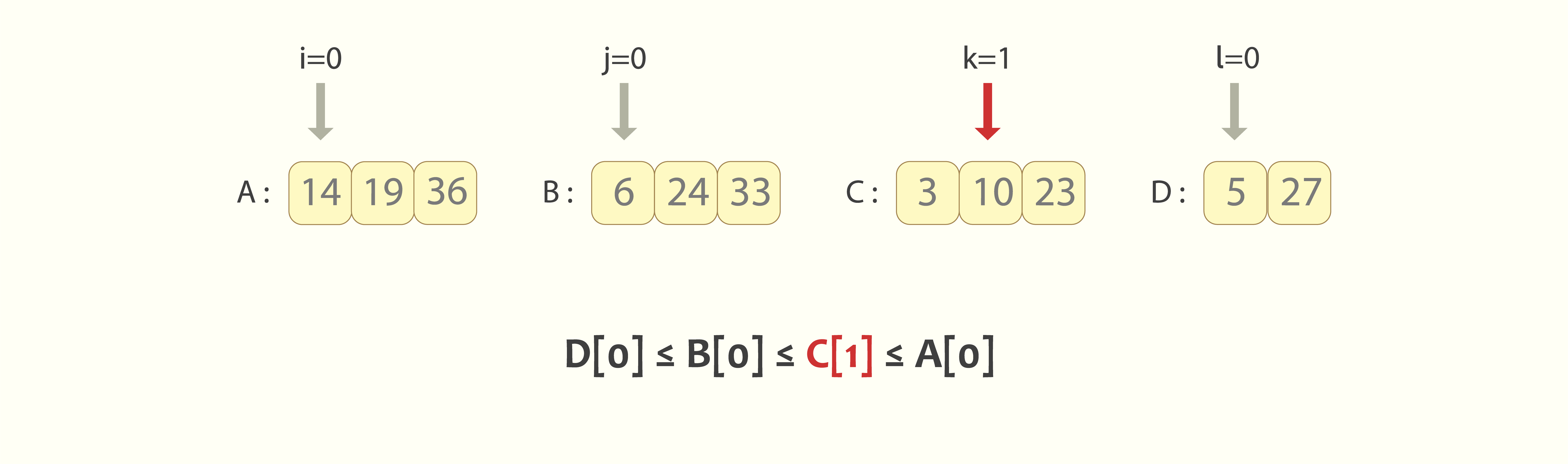
So we made only 2 comparisons and figured out the next relative ordering of head values. This outperforms the K–merge algorithm, where we were doing “K-1=3” comparisons per step.

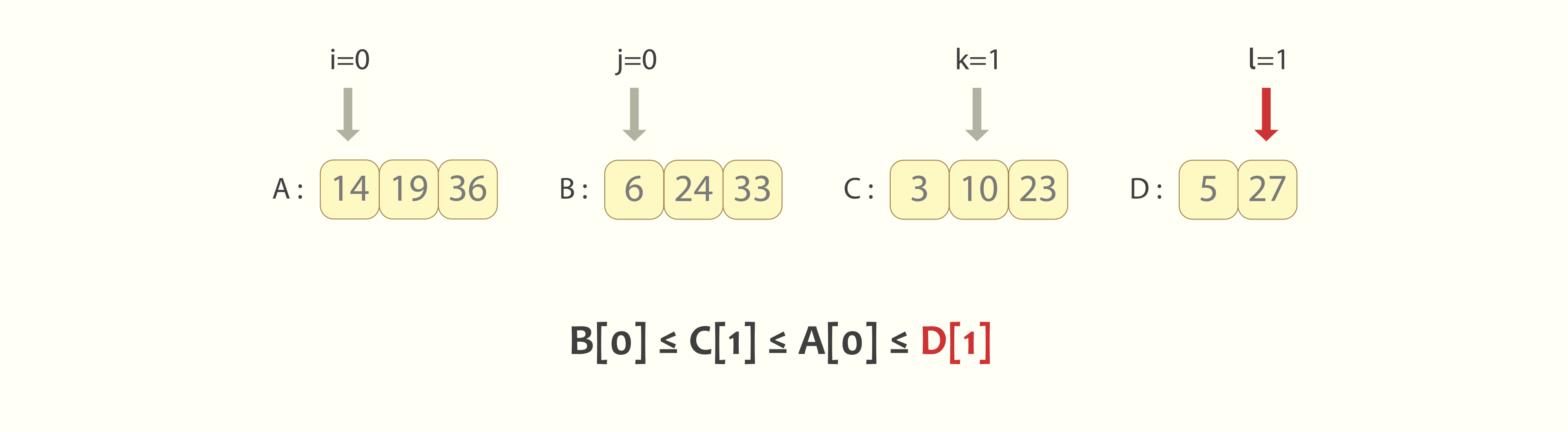
From this point, the algorithm repeats. As the updated relative ordering is “D[0] ≤ B[0] ≤ C[1] ≤ A[0]”, we’ll take the next smallest value “D[0]” to the result sequence, and will properly place its substitution “D[1]” into the remaining sorted list “B[0] ≤ C[1] ≤ A[0]”, to preserve its sorted state. That will require just another 2 comparisons.

···

3. Implementation of guided merge procedure

The idea described above requires keeping track of the sorted list of current head values. For example, at some point in time it can be as:

C[k] ≤ D[l] ≤ B[j] ≤ A[i].

The straightforward way to do that is to keep a short sorted array. Let’s name it “sorted_cursors”.

sorted_cursors[ 4 ] = [ (C[k], C), (D[l], D), (B[j], B), (A[i], A) ]

Note that we will need to store not only the head values themselves, but also references (or pointers) to the sequences from which those values were taken. This is required so we’ll be able to substitute, for example, “C[k]” with “C[k+1]” on the next step, so we will know that the next head value should be taken from the sequence “C”. As we already observed in the previous chapter, once “C[k]” is placed in the result and “C[k+1]” substitutes it, the next 4 possible arrangements of head values are:

• [ (C[k+1], C), (D[l], D), (B[j], B), (A[i], A) ] ,

• [ (D[l], D), (C[k+1], C), (B[j], B), (A[i], A) ] ,

• [ (D[l], D), (B[j], B), (C[k+1], C), (A[i], A) ] , and

• [ (D[l], D), (B[j], B), (A[i], A), (C[k+1], C) ] .

To efficiently maintain such a “sorted_cursors” array, we should left-shift some of its values by one position and place the new pair “(C[k+1], C)” into the emptied slot:

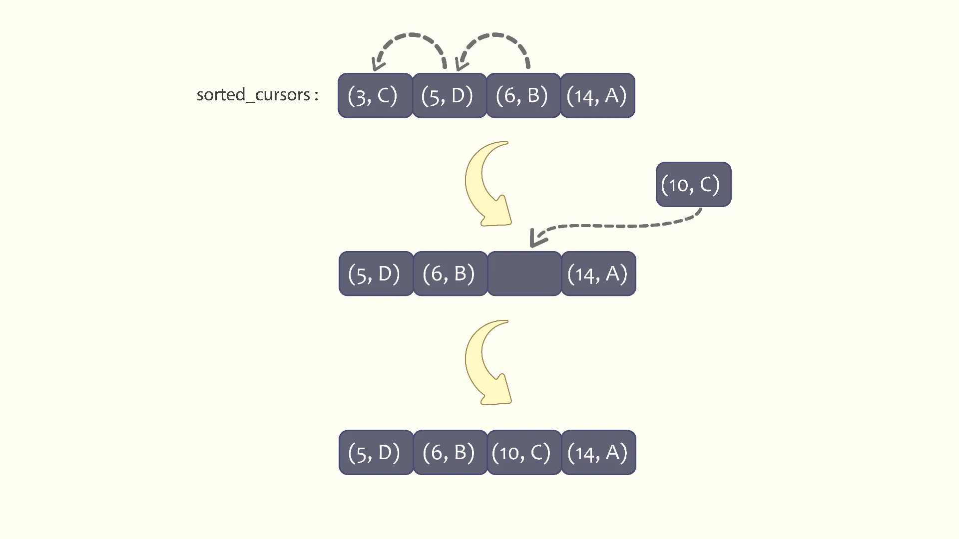
All that is possible and is, in fact, the straightforward way to implement. But that is not the best approach for us, as it introduces several extra assignments per step when doing the left-shifts.

Instead, the guided merge algorithm keeps track of the current sorted sequence of head values by jumping between different fragments of the code. For a given ‘K’, there are “K!” possible arrangements of head values. In our case, as “K=4”, that is “4! = 24” ways:

• “abcd”, (meaning “A[i] ≤ B[j] ≤ C[k] ≤ D[l]”),

• “abdc”, (meaning “A[i] ≤ B[j] ≤ D[l] ≤ C[k]”),

• “acbd”,

• “acdb”,

• “adbc”,

• …

• “dcab”,

• “dcba” (meaning “D[l] ≤ C[k] ≤ B[j] ≤ A[i]”).

Eventually, what I suggest is having a fragment of code for every possible arrangement. For the first possible arrangement “abcd”, that fragment will look like:

/// Performs guided merge of 4 input arrays A[0..n1), B[0..n2), /// C[0..n3) and D[0..n4), writing the merged result into array “Out”.void guided_4_merge( const int A[], int n1, 		const int B[], int n2, 		const int C[], int n3, 		const int D[], int n4, 		int Out[] ) {	int i=0, j=0, k=0, l=0;  // Indexes over the 4 input sequences	int m=0;  // Index over the output sequence	// ...	// ...	// << initial decision of the case, that we will write a bit later >>	// ...	// ...abcd_label:  // Currently “A[i] <= B[j] <= C[k] <= D[l]”	Out[m++] = A[i];  // Place the head of “A” into the result sequence	++i;  // Advance to the next value “A[i+1]”	if ( i == n1 )  // Check if sequence “A” is exhausted		goto finish_label;	// Perform binary search of the new “A[i]” (formerly “A[i+1]”) in the     // remaining sorted list “B[j] <= C[k] <= D[l]”	if ( A[i] <= C[k] ) {		if ( A[i] <= B[j] )			goto abcd_label;  // The ordering has not changed		else			goto bacd_label;  // The ordering is                               // “B[j] <= A[i] <= C[k] <= D[l]” now	}	else {		if ( A[i] <= D[l] )			goto bcad_label;  // The ordering becomes                               // “B[j] <= C[k] <= A[i] <= D[l]”		else			goto bcda_label;  // The ordering becomes                               // “B[j] <= C[k] <= D[l] <= A[i]”abdc_label:  // Currently “A[i] <= B[j] <= D[l] <= C[k]”	// ...	// << similar sequence of instructions for the ordering “abdc” >>	// ...	// ...	// << similar code fragments for the other 22 possible arrangements >>	// ...	// ...	// ...	// << finalization, which we will write a bit later >>	// ...	// ...}

This way, we will have 23 more fragments, each corresponding to another possible arrangement of the current head values “A[i]”, “B[j]”, “C[k]” and “D[l]”. Codes of all those fragments will be isomorphic, which is why in certain programming languages like C or C++, macros can be (and should be) used to avoid duplication of source code.

Having “K!” isomorphic code fragments, and using the “goto” operator to jump between them compensates for the cost of doing left-shifts and insertions into the short array “sorted_cursors”. Note that only one “goto” is enough, compared to several assignments during the left-shift. Another interesting point is that the goto operator becomes irreplaceable if we want to act in the described way.

The presented code also has “finish_label”, where the execution jumps once either of the 4 input sequences is exhausted, and when it remains to merge the tails of the other 3 sequences. Then, as we prefer to continue with the guided merge logic, another “3! = 6” labels must follow, each corresponding to a permutation of identifiers of 3 sequences. Surely, that is preferable to implement as a separate function, like “guided_3_merge”, which is why the ending of our function “guided_4_merge” will look like this:

void guided_4_merge( const int A[], int n1, 		const int B[], int n2, 		const int C[], int n3, 		const int D[], int n4, 		int Out[] ) {	int i=0, j=0, k=0, l=0;  // Indexes over the 4 input sequences	int m=0;  // Index over the output sequence	// ...	// ...	// << initial decision of the case, which we will write a bit later >>	// ...	// ...	// ...	// ...	// << processing of the 24 different orderings of “A, B, C, D” comes here >>	// ...	// ...finish_label:  // Here only 3 sequences remain to merge, and                // we should check which one was exhausted	if ( i == n1 )  // The first sequence ‘A’ is exhausted		return guided_3_merge( B+j, n2-j, C+k, n3-k, D+l, n4-l, Out+m );				// We merge remaining tails of ‘B’, ‘C’, and ‘D’, 				// which are now ‘n2-j’, ‘n3-k’, and ‘n4-l’-long 				// respectively.	else if ( j == n2 )  // The second sequence ‘B’ is exhausted		return guided_3_merge( A+i, n1-i, C+k, n3-k, D+l, n4-l, Out+m );	else if ( k == n3 )  // The third sequence ‘C’ is exhausted		return guided_3_merge( A+i, n1-i, B+j, n2-j, D+l, n4-l, Out+m );	else // The fourth sequence ‘D’ is exhausted		return guided_3_merge( A+i, n1-i, B+j, n2-j, C+k, n3-k, Out+m );}

Finalizing the code of “guided_4_merge“, before the first jump to one of the 24 different labels, we need to understand which label it will be. In other words, we need to figure out the relative ordering of the initial head values A[0], B[0], C[0], and D[0]. That can be done with manual comparisons, like this:

void guided_4_merge( const int A[], int n1, 		const int B[], int n2, 		const int C[], int n3, 		const int D[], int n4, 		int Out[] ) {	int i=0, j=0, k=0, l=0;  // Indexes over the 4 input sequences	int m=0;  // Index over the output sequence	// Comparing the 4 head values A[0], B[0], C[0] and D[0], to 	// figure out the initial relative ordering, and jump right there.	if ( A[0] < B[0] ) {		if ( B[0] < C[0] ) {			if ( C[0] < D[0] )				goto abcd_label;			else				...		}		else {			if ( B[0] < D[0] )				goto acbd_label;			else				...		}	}	else {		...	}	// ...	// ...	// << processing of the 24 different orderings of “A, B, C, D” comes here >>	// ...	// ...	// ...	// ...	// << finalization, when we merge 3 remaining tails >>	// ...	// ...}

Another macro can be (and should be) used to avoid inflation of the beginning part of “guided_4_merge”. Note that the initial decision of relative ordering is made only once.

The complete code for the guided merge procedures in C++, for the cases “K=3” and “K=4”, is available on my GitHub at [5].

As we already noted, the presented approach will not be practical for large values of ‘K’, as ‘K!’ increases faster than any exponent. But it is completely practical when “K=3” or “K=4”, as the number of possible orderings is “3! = 6” and “4! = 24”, respectively. Note that if “K=2”, the guided merge procedure downgrades to ordinary merge.

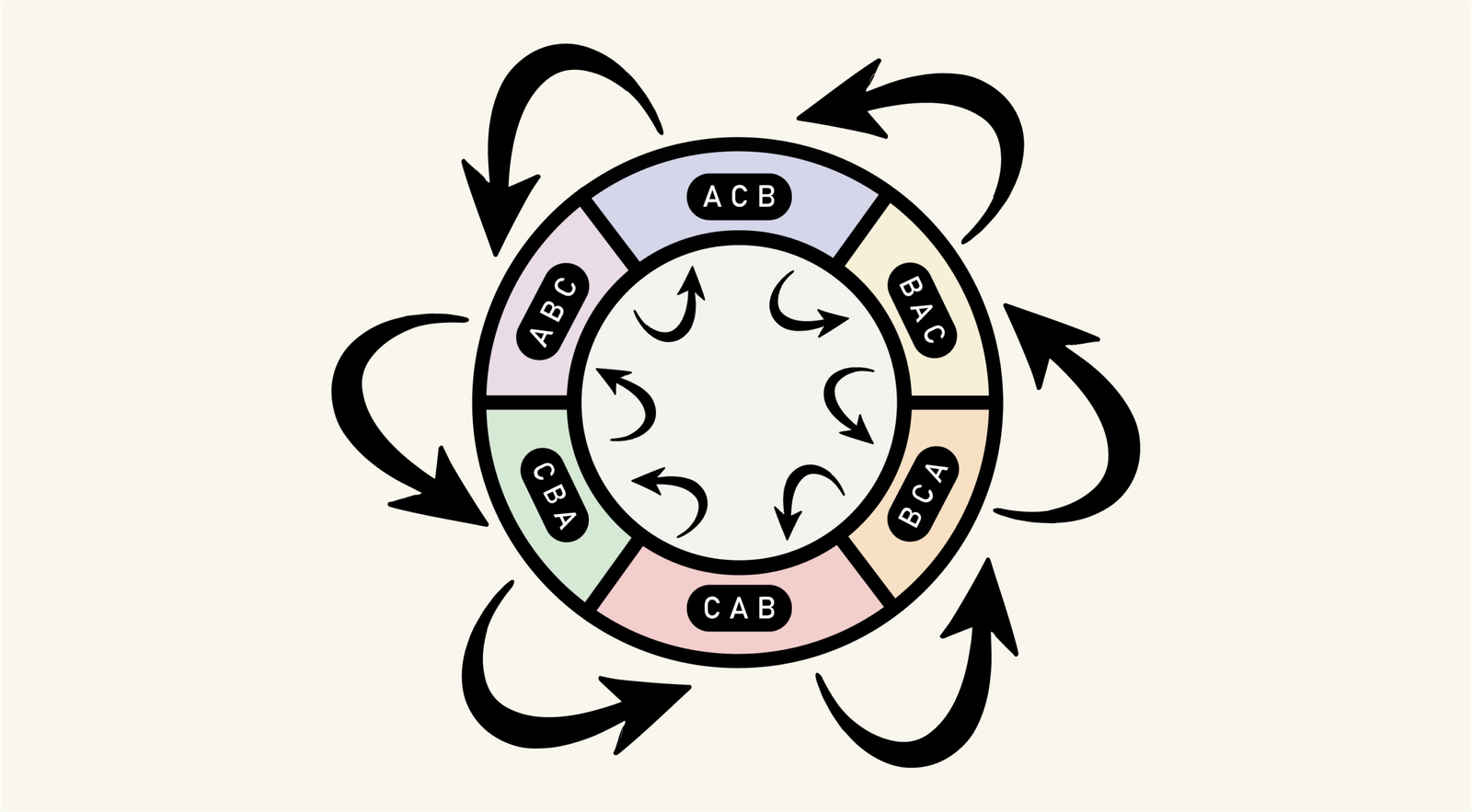
Before finishing this chapter, I want to add the diagram of possible jumps over the “3! = 6” labels, for the case “K=3”:

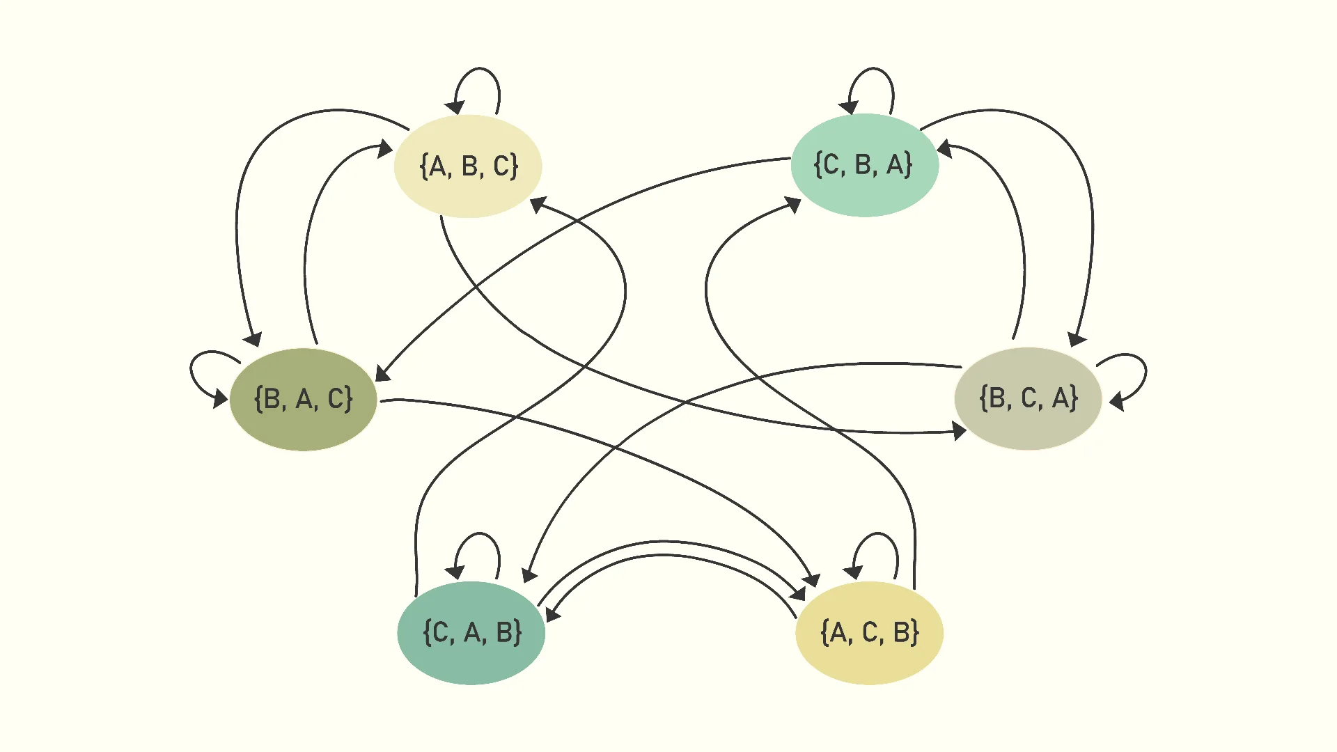
We see that, while on any label, only 3 of the 6 labels can become the next ones. For the case “K=4”, while on any label, only 4 of the 24 labels can become the next ones. That is why we can expect a practical advantage of guided K-merge over ordinary K-merge.

I named the algorithm “guided merge” because the impression is that we constantly guide its execution over all possible orderings of the ‘K’ head values. We are always aware not only of the next smallest head value, but also of their relative arrangement.

···

4. The guided merge sort algorithm

Once the guided K-merge procedure is derived, we can introduce guided merge sort as a general-purpose sequence sorting algorithm. Guided merge sort (or, more precisely, guided K-merge sort) is a recursive algorithm and relies on the guided merge (more precisely, guided K-merge) procedure, exactly the same way that ordinary merge sort is a recursive algorithm and relies on the merge procedure.

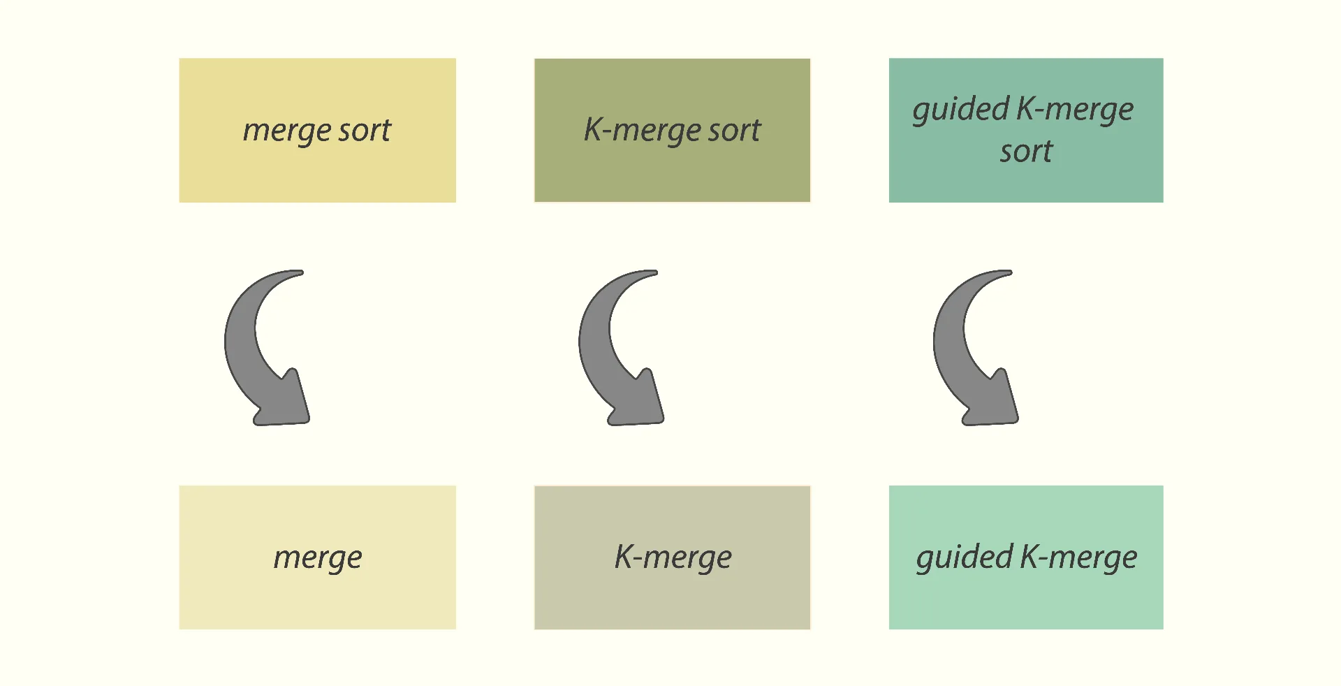
The logic of guided K-merge sort is:

• divide the input sequence into ‘K’ equal parts,

• recursively sort each of them by invoking the same guided K-merge sort algorithm,

• combine the result ‘K’ sorted sequences into one, using the guided K-merge procedure.

We can already write the code of the guided K-merge sort algorithm in C++:

/// Sorts the n-long array ‘X’, in an increasing order.void guided_4_merge_sort( int X[], int n ) {	// Check exit branch at first, as this is a recursive function.	if ( n < 16 ) {		// According to a common practice of various sorting 		// algorithms, here also we switch to Insertion sort when 		// the length of sub-array becomes small enough.		insertion_sort( X, n );		return;	}	// Otherwise, divide the n-long range in 4 equal parts	const int quarter = n / 4;	// Recursively sort each part	//    Note, because of the rounding in division by 4, the last part 	//    might result in a shorter length.	guided_4_merge_sort( X, quarter );	guided_4_merge_sort( X+quarter, quarter );	guided_4_merge_sort( X+2*quarter, quarter );	guided_4_merge_sort( X+3*quarter, n-3*quarter );	// Temporarily allocate a buffer for storing the result of the merge.	//    Note, in an optimal implementation it makes sense to allocate 	//    buffer only once, and use it in every recursive call. We just 	//    don’t do that here for simplicity.	int* buffer = new int[ n ];	// Merge the 4 sorted arrays into one, using “guided merge” algorithm	guided_4_merge( X, quarter, 			X+quarter, quarter, 			X+2*quarter, quarter, 			X+3*quarter, n-3*quarter, 			buffer );	// Copy back the merged sequence from buffer to original array	//   Note, in an optimal implementation we should use ping-pong 	//   merge sort, thus merging the data to buffer on even levels 	//   of recursion, and merging it back from buffer to ‘X’ on 	//   the odd levels of recursion. That significantly reduces the 	//   time spent on copying-back from buffer. We just don’t do it 	//   either, for simplicity purposes.	std::copy_n( buffer, n, X );	delete [] buffer;}

As we see, the code is almost identical to that of K-merge sort. The only difference is that instead of “_4_merge”, the “guided_4_merge” procedure is called to combine the 4 sorted sub-arrays.

As guided K-merge sort is a recursive algorithm that calls itself on shorter sub-arrays, in the first 10 lines there is the exit branch. Once the current sub-array becomes shorter than 16, we switch to insertion sort. This is a common practice and is used in many other sorting algorithms, such as introsort or timsort.

Next, at lines 12-19 we divide the n-long input sequence into 4 equal parts. The last part might result a bit shorter because of the rounding in integer division. Then, we recursively call guided_4_merge_sort on each of those parts, and sort them independently from each other.

Finally, at lines 20-39 we combine (i.e., merge) the 4 sorted arrays back into one, using the “guided_4_merge” procedure. To not overcomplicate the code here, first we merge them into a temporary ‘buffer’, and then copy the result back to the input array ‘X’. This copying back can be highly optimized using the ping-pong merge sort approach.

Also, in an optimized implementation, it makes sense to allocate the ‘buffer’ only once, and provide it to every call of “guided_4_merge_sort” as an extra argument. I just decided not to do that either, to keep the code here as simple as possible.

The time complexity of guided K-merge sort is identical to that of K-merge sort, and equals O(n log n).

The complete and highly optimized implementation of guided K-merge sort for the cases of “K=3” and “K=4” can be found on my GitHub at [5].

···

5. Theoretical evaluation

In this chapter, we will do a theoretical comparison between guided K-merge sort and K-merge sort algorithms.

As the logic of those two functions is identical, if there are any reasons for guided_k_merge_sort to outperform k_merge_sort, then those are the same reasons by which guided_k_merge outperforms k_merge. That’s why we’ll concentrate only on the latter comparison.

Evaluation of K-merge

Assuming there are ‘K’ sorted sequences, k_merge repeatedly finds the next smallest head value of them and places it into the output sequence. So, if lengths of those sequences are:

n₁, n₂, …, n_K,

which in total gives the length of:

n = n₁ + n₂ + … + n_K,

then exactly ‘n’ steps will be required to process them all, and copy (or move) each of their value to the output.

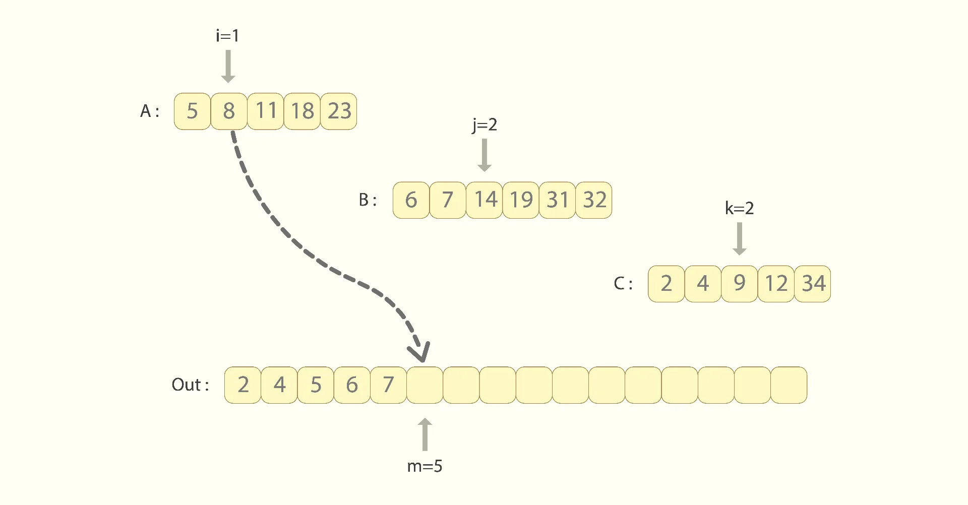
At every step, k_merge sequentially scans the current heads of all the ‘K’ sequences, looking for the next smallest one. That requires ‘K-1’ comparisons. After the next smallest head is found, one assignment is done to move it to the output. So the number of operations performed during k_merge is:

“n*(K-1)” comparisons,
“n” assignments.

Here we neglect the fact that in some cases, most values of some sequence(s) can be greater than all values of the other sequence(s). In such a case, the other sequences will be exhausted much sooner, leaving us with only ‘K-1’ (or even fewer) sequences to merge, thus requiring fewer comparisons to be done later. I guess we can skip such scenarios here, because if there is no dependency between values of the input, their probability is very small.

Evaluation of guided K-merge

The outcome of guided K-merge is identical to that of K-merge, as both algorithms copy (or move) all the ‘n’ values to the output. So, in a general case, guided K-merge also performs ‘n’ steps to make all those copies.

However, guided K-merge also keeps track of the relative order of the ‘K’ current head values.

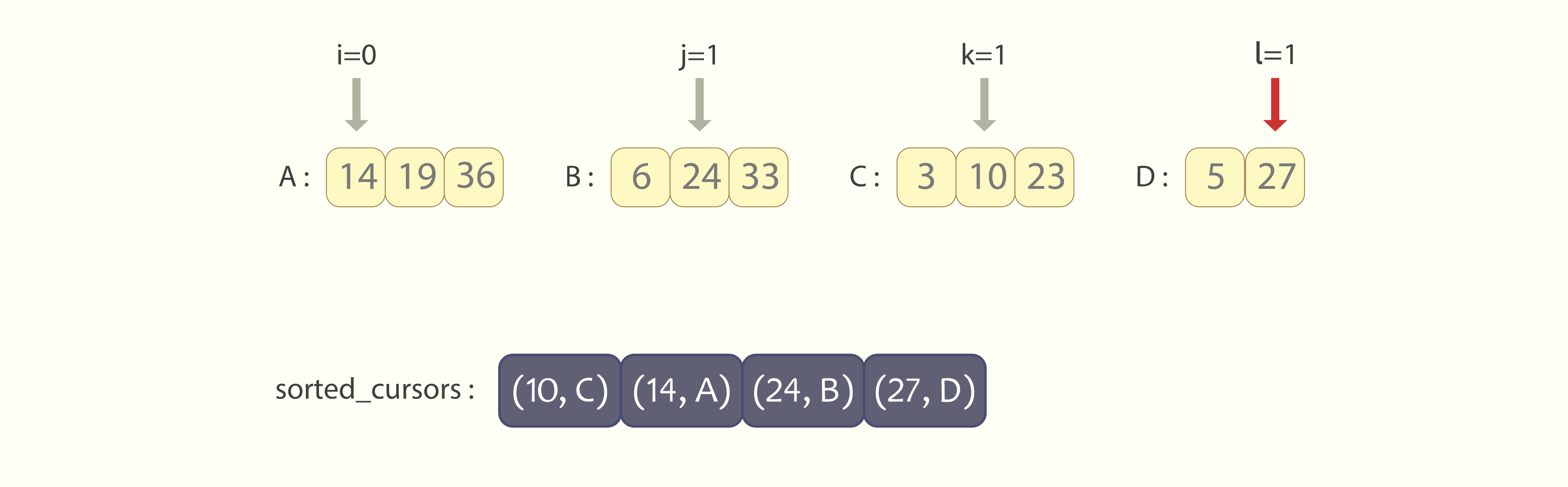
As we figured out in the previous chapter, instead of keeping the physical array “sorted_cursors” in memory, different arrangements of its values will correspond to different sections in the code. Jumps between those sections are performed with the goto operator.

Now what guided K-merge does on every step is:

• picks the next smallest head value, as the first one of the current arrangement,

• places it into the output [requires 1 assignment],

• substitutes it with the next value from the same sequence [requires a binary search in the “K-1”-long sorted list, thus, “log₂K” comparisons],

• jumps to possibly another section, which corresponds to the next arrangement of head values [requires one “goto” invocation].

Summarising, the overall number of operations performed by guided K-merge is:

• “n*log₂K” comparisons,

• “n” assignments,

• “n” jumps.

As in the evaluation of K-merge, here we also neglect the probability that one of the ‘K’ input sequences might exhaust much sooner, leaving us with “K-1” (or even fewer) sequences to merge. If the input values are distributed uniformly, the probability of such a scenario is very small.

We also neglect the cost of figuring out the initial arrangement of head values “A[0]”, “B[0]”, “C[0]”, …, as that is performed only once per guided K-merge.

Comparison between K-merge sort and guided K-merge sort

Comparing K-merge and guided K-merge algorithms results in the following table:

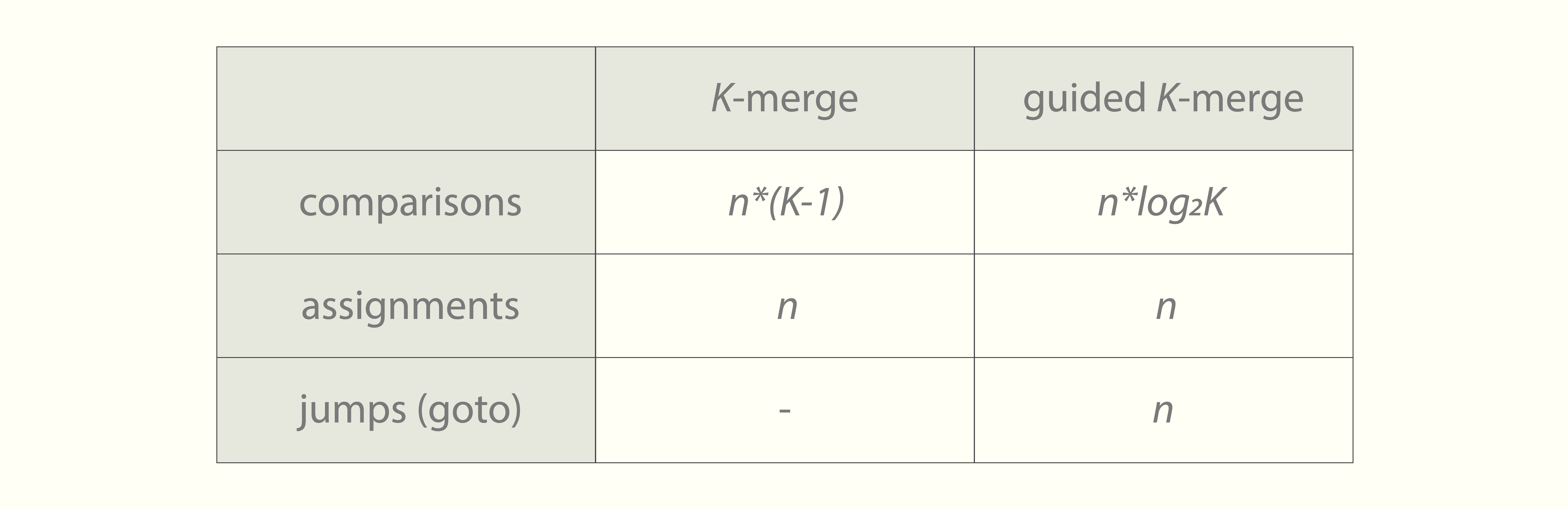
We see that guided K-merge performs fewer comparisons. That advantage becomes more significant as the value of ‘K’ increases. At the same time, introducing too large value for ‘K’ will result in “K!” isomorphic fragments of code, which will both inflate the code size and almost certainly cause cache misses when jumping between them; thus, will significantly increase the runtime. On the other hand, introducing a very small value for ‘K’, like “K=2”, will downgrade the guided K-merge algorithm into ordinary merge.

Considering that the sorting algorithms are recursive with depth of “log_Kn”, the comparison between K-merge sort and guided K-merge sort results in:

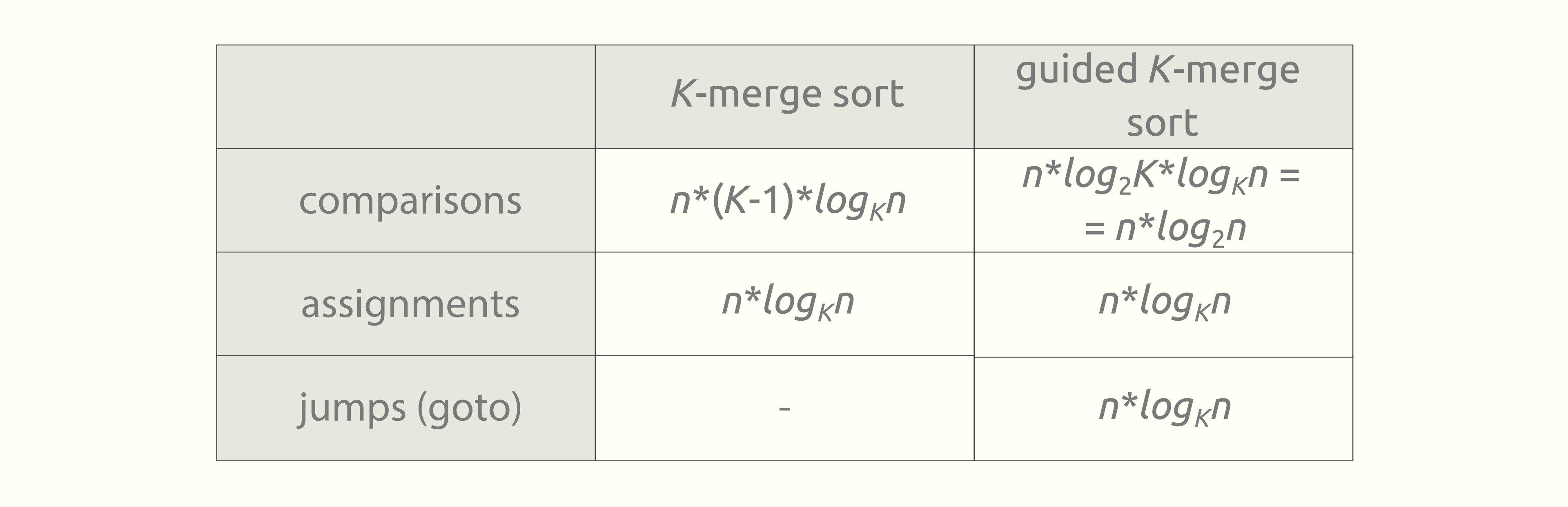
In the next section, we will experimentally figure out the optimal value of ‘K‘ to keep the right balance between the mentioned factors.

···

6. Practical evaluation

In this chapter, we’ll observe results of experimental comparison. The following sorting algorithms, all implemented in C++, were benchmarked on randomly generated arrays:

• STL’s standard sorting routine – “std::sort”,

• STL’s heap sort – “std::make_heap”, followed by “std::sort_heap”,

• ordinary merge sort,

• ordinary merge sort, that uses guided 2-merge underlying routine,

• 3-merge sort,

• guided 3-merge sort,

• 4-merge sort,

• guided 4-merge sort.

The experiments were different from each other in:

• ‘n’ – length of the array being sorted,

• types of objects in the array,

• ‘switch_threshold’ – different thresholds for sub-array length, when during the last stages of recursion merge sort implementations switch to insertion sort,

• arrays containing lots of / few repeated values.

All the experiments were performed under the following machine & environment:

• Hardware: Alienware m15 R6, 11th Gen Intel® Core™ i7-11800H × 16, 16.0 GiB RAM

• Operating system: Ubuntu 26.04 LTS, Linux 7.0.0-28-generic #28-Ubuntu SMP PREEMPT_DYNAMIC x86_64 GNU/Linux

• Compiler: g++ 15.2.0

• Compiler flags: -Wall -Wextra -std=c++17 -DNDEBUG -O3

• Benchmark library: Google Benchmark 1.9.1-1build1

All the C++ code on which benchmarking was performed can be found at [5].

Summary of the results

All experimental results can be summarised in the following statements:

• All of the times, STL heap sort performs slower than std::sort.

  • Explanation: This is quite expected, as std::sort implements the introsort algorithm, which is a hybrid approach that combines quick sort, heap sort, and insertion sort in the best possible manner.

• Ordinary merge sort that relies on the guided 2-merge routine is a bit slower than the ordinary merge sort that relies on the standard merge routine.

  • Explanation: An expected outcome, because the code of the guided 2–merge procedure contains 2 goto instructions, in contrast to the code of the standard merge procedure. While theoretically both codes perform exactly the same actions, modern CPUs are highly optimised for parallelising and vectorising ordinary loops, and not goto jumps.

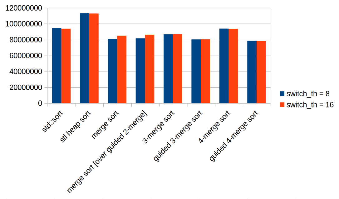
• When sorting primitive data types (32-bit or 64-bit integers or floating-point numbers), std::sort outperforms all other candidate algorithms, including variants of guided merge sort.

  • Explanation: Repetitive comparisons and assignments of primitive variables are highly optimised on modern CPUs. Within guided K-merge sort, the cost of jumps between code fragments as well as the inability of the hardware to vectorise or parallelise such a code, surpasses its theoretical advantages of making less operations on primitive data types.

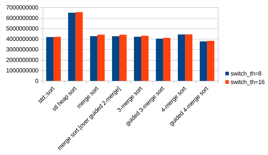
• When sorting large objects (150-500 long static or dynamic arrays of primitive data types), 3-merge sort performs slower than ordinary merge sort, and 4-merge sort performs even slower.

  • Explanation: This is expected and can be observed purely from theoretical evaluation. With the growth of ‘K’, the number of comparisons grows linearly.

• When sorting the same large objects, guided 3-merge sort outperforms both ordinary merge sort and std::sort, while guided 4-merge sort outperforms them all even more.

  • Explanation: This is the advantage of the guided K-merge sort algorithm over others, including ordinary merge sort, and even STL’s standard std::sort. Such a result is also expected from the theoretical evaluation. Within guided K-merge sort, with the growth of ‘K’, the number of comparisons remains the same – “n*log₂n”, while the number of assignments drops, being equal to “n*log_Kn”. When sorting large objects, the majority of the time goes on comparing and assigning them to each other, so the time spent on jumps between code fragments, as well as the inability of the CPU to vectorise operations, are compensated. That is why in this scenario, practical evaluation turns out alike the theoretical evaluation.

Benchmarking

Here are the timings of sorting 150-long dynamic arrays of 64-bit integers. Length of the sequence being sorted is “n = 50’000”:

And here are the timings of sorting 250-long static arrays of 64-bit integers. The length of the sequence being sorted is “n = 750’000” now:

···

7. Conclusion

In the current article, I have described the guided K-merge procedure and have derived the guided K-merge sort general-purpose sorting algorithm.

The novelty here is in how the ‘K’ sorted sequences are being merged into one. In contrast to ordinary merge or K-merge procedures, guided K-merge doesn’t keep any helper information in containers, and instead uses “K!” isomorphic fragments of code, and jumps between them with the goto operator.

This efficiently reduces the number of operations performed per step, making only ”log₂K” comparisons, instead of the “K-1” comparisons of the K-merge procedure.

The drawback of guided K-merge is that “K!” isomorphic fragments appear in the code. So, to avoid inflating the size of the program, picking values “K=3” or “K=4” promises the best balance between performance and the memory used.

Implementation of the guided K-merge sort algorithm in C++ for cases “K=3” and “K=4” can be found on my GitHub at [5].

If you’ll have any suggestions, questions, or will spot a mistake in the text, feel free to contact me by LinkedIn (the link below).

Thank you so much for reading till the end!

···

My gratitude to:

• Elen Grigoryan, for careful design of all used illustrations (behance.net/elengrigoryansun),

• Meri Movsesyan, for detailed review of the article’s draft (linkedin.com/in/mermovs/).

If you enjoyed this article, feel free to contact me on LinkedIn (linkedin.com/in/tigran-hayrapetyan-cs/).

All the images were designed upon request of the author.

···

References

[1] – Sorting Algorithms, Part 1: Merge Sort, by Vyacheslav Efimov: https://towardsdatascience.com/merge-sort-explained-and-visualised-660f6946d9b5/

[2] – Making Sense of Merge Sort [Part 1], by Vaidehi Joshi: https://medium.com/basecs/making-sense-of-merge-sort-part-1-49649a143478

[3] – “Learn Merge Sort in 13 minutes”, by BroCode: https://www.youtube.com/watch?v=3j0SWDX4AtU

[4] – “Direct k-way merge”: https://en.wikipedia.org/wiki/K-way_merge_algorithm#Direct_k-way_merge

[5] – Implementation and benchmarking of guided K-merge sort in C++: https://github.com/tigranh/guided_merge_sort